一些矩阵乘法

矩阵乘法是线性代数中一种基本且重要的运算，它在众多领域如计算机科学、物理学、工程学等都有广泛应用。

基本矩阵乘法

对于两个矩阵\(A\)和\(B\)，要进行矩阵乘法\(AB\)，要求矩阵\(A\)的列数等于矩阵\(B\)的行数。假设\(A\)是一个\(m \times n\)的矩阵，\(B\)是一个\(n \times p\)的矩阵，那么它们的乘积\(AB\)是一个\(m \times p\)的矩阵。其元素计算方式为：

\[(AB)_{ij} = \sum_{k = 1}^{n} a_{ik}b_{kj} \]

其中\(i = 1, \cdots, m\)，\(j = 1, \cdots, p\)。

例如，若

\[A = \begin{bmatrix}1&2\\3&4\end{bmatrix} \quad B = \begin{bmatrix}5&6\\7&8\end{bmatrix} \]

这里\(A\)是\(2 \times 2\)矩阵，\(B\)是\(2 \times 2\)矩阵，满足相乘条件。\(AB\)的元素计算如下：

\[\begin{align*} (AB)_{11} &= 1\times5 + 2\times7 = 5 + 14 = 19\\ (AB)_{12} &= 1\times6 + 2\times8 = 6 + 16 = 22\\ (AB)_{21} &= 3\times5 + 4\times7 = 15 + 28 = 43\\ (AB)_{22} &= 3\times6 + 4\times8 = 18 + 32 = 50 \end{align*} \]

所以\(AB = \begin{bmatrix}19&22\\43&50\end{bmatrix}\)。

矩阵乘法不满足交换律，即一般情况下\(AB \neq BA\)，并且它满足结合律\((AB)C = A(BC)\)以及分配律\(A(B + C) = AB + AC\)和\((B + C)A = BA + CA\)。
矩阵乘法本质上是线性变换的表示形式，更多细节可以参考线代/高代。

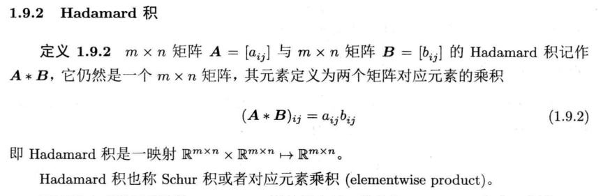
哈达玛积（Hadamard product）

定义

例：

\[\left[ \begin{matrix} 1 & 2 \\ 3 & 4 \end{matrix} \right] \circ \left[ \begin{matrix} 5 & 6 \\ 7 & 8 \end{matrix} \right] = \left[ \begin{matrix} 1*5 & 2*6 \\ 3*7 & 4*8 \end{matrix} \right]\]

---

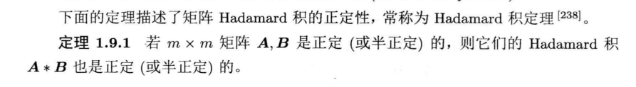
证明：

考虑对\(A,B,A \circ B\)二次型展开即可

---

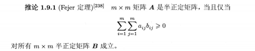
证明：
必要性：由定理1.9.1，对\(A*B\)二次型展开，即考虑\(x^T(A \circ B)x\)，其中x取全1向量得证。
充分性：反证法。假设\(A\)不是半正定的，存在非零向量\(x_0使得x_0^TAx_0<0\),构造半正定矩阵\(B_0=x_0x_0^T\),有

\[\sum_{i = 1}^{m}\sum_{j = 1}^{m}a_{ij}(b_0)_{ij}=x_0^TAx_0<0 \]

矛盾，得证。

---

一些性质

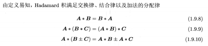
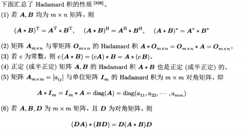
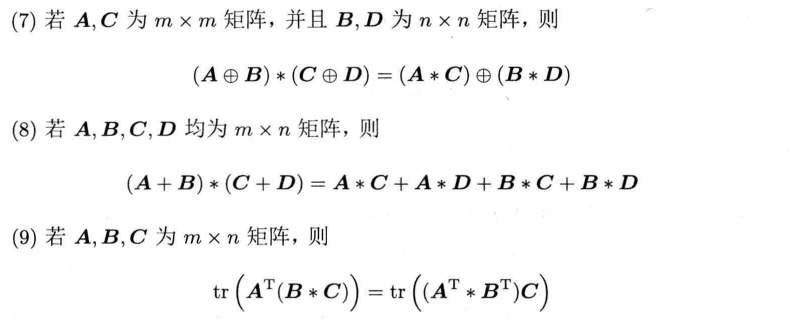
(9)证明：

\[(A^T(B \circ C))_{ii} = \sum_{h}a_{hi}(b_{hi}c_{hi}) = \sum_{h}(a_{hi}b_{hi})c_{hi} = ((A^T \circ B^T)C)_{ii} \]

对角元相等因此迹相等。
关于迹性质在一些优化问题里对矩阵求导里面可能用到。

---

Hadamard积服从的不等式

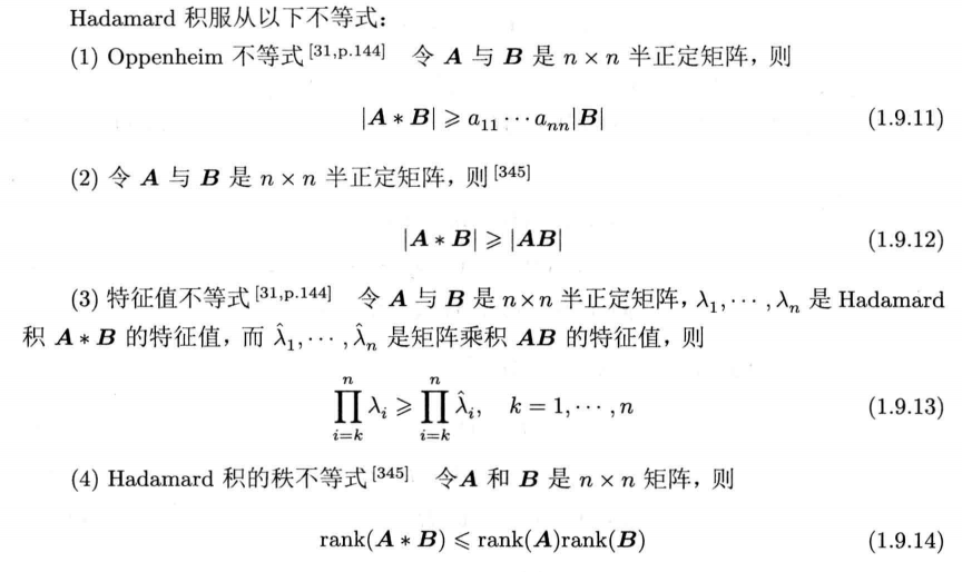
证明：
（1）推（2）： 注意到当B为单位阵时有\(|A| = b_{11}...b_{nn}|A| \le |E \circ A| = a_{11}...a_{nn}\)，即hadamard不等式\(|A| \le a_{11}...a_{nn}\)。且\(|AB| = |A||B|\)，所以，\(|A \circ B| \ge a_{11}...a_{nn}|B| \ge |A||B|\)。
（2）推（3）：由（2）显然。
（4）：对\(A \circ B，A,B\)列分块可得到\(A \circ B\) 可以被A和B共同组成的列向量线性表出。

---

一些用法

1. 矩阵求导
2. 图像增强，对图像原矩阵做点运算
   比如使用HIS（Hue, Intensity, Saturation）彩色图像模型得到图像的I亮度矩阵，通过hadamard积可以对图像亮度增强或者减弱。
3. 高通/低通滤波器，对图像的频率域矩阵做点运算
   图像处理中往往会通过二维离散傅里叶变换把图像转化到频域上处理，类似一维傅里叶变换，变换后的向量是对称的。低频信息位于0对称轴附近而高频信息在两侧。二维傅里叶变换得到的图像频域也是低频信息在中间而高频信息在四周。并且高频信息代表图像的细节部分而低频信息代表图像的整体信息。构建一种简单的高通滤波器（中心为0，四周全1的矩阵）或者低通滤波器（中心为1，四周全0的矩阵），分别做hadamard积可以选择性的保留图像的细节或整体信息。
4. 卷积
   卷积，toeplitz矩阵与FT。

克罗内克积（Kronecker Product）

定义

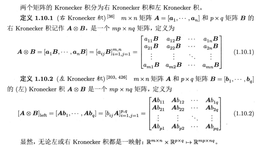
一般采用的是右Kronnecker积。Kronnecker积也被看作是一种张量积。

一些性质

由于Kronecker积本质上也是元素间相乘，所以同样存在结合律与分配律。对于任意矩阵X、Y与Z，有：

\[X \otimes (Y \otimes Z) = (X \otimes Y) \otimes Z \tag{1} \]

\[X \otimes (Y + Z) = X \otimes Y + X \otimes Z \tag{2} \]

但根据定义显然不满足交换律。

对于任意矩阵\(X∈R_{m×n}、Y∈R_{s×t}、U∈R_{n×p}\)与\(V∈R_{t×q}\)，则矩阵\(X⊗Y∈R(ms)×(nt)\)的列数\(nt\)与矩阵\(U⊗V∈R(nt)×(pq)\)的行数\(nt\)一致，可进行矩阵相乘。而且有以下常用性质（重要）：

\[(X \otimes Y)(U \otimes V) = XU \otimes YV \tag{*} \]

根据定义展开即可证明

两个推论:

\[(A \otimes B)^{-1} = A^{-1} \otimes B^{-1} \tag{1} \]

所以计算K积的逆可以先取逆再取K积。
当\(A∈R_{m×m}、B∈R_{n×n}\)时

\[A \otimes B = (A \otimes E_{n})(B \otimes E_{m}) = (B \otimes E_{m})(A \otimes E_{n}) \tag{2} \]

类似\((1)\)，还有\((A \otimes B)^{H} = A^{H} \otimes B^{H}\)，即对共轭转置分配。

---

此外，K积的迹，范数，行列式，秩满足下列性质：

\[\begin{aligned} tr(A \otimes B) &= tr(A)tr(B) \\ ||A \otimes B||_F &= ||A||_F||B||_F \\ det(A_{m \times m} \otimes B_{n \times n}) &= det(A)^ndet(B)^m \\ rank(A \otimes B) &= rank(A)rank(B) \\ \end{aligned} \]

特别的，如果有\(A\in \mathbb{R}^{m \times m},B\in \mathbb{R}^{n \times n}\)，那么\(A \otimes B\)对应的特征值和特征向量分别为\(\lambda_i*\mu_j\)和\(x \otimes y\)，如果有\(Ax=\lambda_ix,By=\mu_jy\)，表明 Kronecker 积的特征值是原矩阵特征值的乘积。利用\((*)\)式可证。

---

Kronecker 积的奇异值分解有如下性质，如果有\(A=U_1 \Sigma_1 V^T_1,B=U_2 \Sigma_2 V^T_2\),那么有\(A \otimes B\)的奇异值分解为：

\[A \otimes B = (U_1 \otimes U_2) (\Sigma_1 \otimes \Sigma_2) (V^T_1 \otimes V^T_2) \]

同样利用\((*)\)式可证。

向量化 (Vectorization)

矩阵向量化就是把矩阵拉直成一个向量，记为\(vec(A)\)，即把矩阵A的每一列堆叠构成一个新的列向量，例：

\[\begin{aligned} vec(A) &= [a_{11},a_{21},...,a_{(m-1)n,a_{mn}}]^T \\ A &= \begin{bmatrix} 1 & 2 \\ 3 & 4 \end{bmatrix} \\ vec(A) &= [1 \quad 3 \quad 2 \quad 4]^T \end{aligned} \]

向量化与矩阵的Kronecker积有一定的关系(和张量的矩阵化相似)，同时对加法和速乘封闭且满足线性关系。
当\(A \in \mathbb{R}^{m \times n},B \in \mathbb{R}^{n \times p},C \in \mathbb{R}^{p \times q}\)时，有以下（1）式：

\[vec(ABC) = (C^T \otimes A)vec(B) \tag{1} \]

由此有推论，当\(A \in \mathbb{R}^{m \times m},B \in \mathbb{R}^{m \times n},C \in \mathbb{R}^{n \times n}\)时，满足：

\[vec(AB) = (I_n \otimes A)vec(B) \tag{2} \]

\[vec(BC) = (C^T \otimes I_m)vec(B) \tag{3} \]

通过矩阵向量化可以用来求解一些矩阵方程如\(\sum_{i}A_iXB_i=C\)，再得到\(vec(X)\)后通过\(reshape(vec(X),m,n)\)得到结果矩阵X。

以及一些最优化问题中目标函数的矩阵形式不方便求解的时候可以转化为向量，把目标函数的参数变成向量的形式，方便求解。（对于张量来说，矩阵化也是简化目标函数的方法）。

Khatri-Rao积

以Kronecker积为基础，可定义另一种十分重要的运算，即Khatri-Rao积。给定任意矩阵

\[X = \begin{bmatrix} | & | & & | \\ x_1 & x_2 & \cdots & x_d \\ | & | & & | \end{bmatrix} \in \mathbb{R}^{m \times d} \quad Y = \begin{bmatrix} | & | & & | \\ y_1 & y_2 & \cdots & y_d \\ | & | & & | \end{bmatrix} \in \mathbb{R}^{n \times d} \]

X与Y的Khatri-Rao积为：

\[X \odot Y = \begin{bmatrix} | & | & & | \\ x_1 \otimes y_1 & x_2 \otimes y_2 & \cdots & x_d \otimes y_d \\ | & | & & | \end{bmatrix} \in \mathbb{R}^{mn \times d} \]

X与Y的Khatri-Rao积的列向量是X和Y的列向量分别做Kronecker积得到的。Khatri-Rao积得到的实际上是Kronecker积得到的线性变换的子空间变换。

参考

[1]Matrix Differential Calculus with Applications in Statistics and Econometrics
[2]矩阵分析与应用 (张贤达著)