Neural Networks and Deep Learning（week3）Planar data classification with one hidden layer(基于单隐藏层神经网络的平面数据分类)

Planar data classification with one hidden layer

你会学习到如何：

• 用单隐层实现一个二分类神经网络

• 使用一个非线性激励函数，如 tanh

• 计算交叉熵的损失值

• 实现前向传播和后向传播

1 - Packages(导入包)

需要导入的包：

• numpy：Python中的常用的科学计算库
• sklearn：提供简单而高效的数据挖掘和数据分析工具
• matplotlib：Python中绘图库
• testCases： 提供了一些测试例子来评估函数的正确性
• planar_utils： 提供各种有用的在这个任务中使用的函数

# Package imports
import numpy as np
import matplotlib.pyplot as plt
from testCases import *
import sklearn
import sklearn.datasets
import sklearn.linear_model
from planar_utils import plot_decision_boundary, sigmoid, load_planar_dataset, load_extra_datasets

%matplotlib inline

np.random.seed(1) # set a seed so that the results are consistent

% testCases.py 保存在本地

```python
import numpy as np

def layer_sizes_test_case():
    np.random.seed(1)
    X_assess = np.random.randn(5, 3)
    Y_assess = np.random.randn(2, 3)
    return X_assess, Y_assess

def initialize_parameters_test_case():
    n_x, n_h, n_y = 2, 4, 1
    return n_x, n_h, n_y

def forward_propagation_test_case():
    np.random.seed(1)
    X_assess = np.random.randn(2, 3)

    parameters = {'W1': np.array([[-0.00416758, -0.00056267],
        [-0.02136196,  0.01640271],
        [-0.01793436, -0.00841747],
        [ 0.00502881, -0.01245288]]),
     'W2': np.array([[-0.01057952, -0.00909008,  0.00551454,  0.02292208]]),
     'b1': np.array([[ 0.],
        [ 0.],
        [ 0.],
        [ 0.]]),
     'b2': np.array([[ 0.]])}

    return X_assess, parameters

def compute_cost_test_case():
    np.random.seed(1)
    Y_assess = np.random.randn(1, 3)
    parameters = {'W1': np.array([[-0.00416758, -0.00056267],
        [-0.02136196,  0.01640271],
        [-0.01793436, -0.00841747],
        [ 0.00502881, -0.01245288]]),
     'W2': np.array([[-0.01057952, -0.00909008,  0.00551454,  0.02292208]]),
     'b1': np.array([[ 0.],
        [ 0.],
        [ 0.],
        [ 0.]]),
     'b2': np.array([[ 0.]])}

    a2 = (np.array([[ 0.5002307 ,  0.49985831,  0.50023963]]))
    
    return a2, Y_assess, parameters

def backward_propagation_test_case():
    np.random.seed(1)
    X_assess = np.random.randn(2, 3)
    Y_assess = np.random.randn(1, 3)
    parameters = {'W1': np.array([[-0.00416758, -0.00056267],
        [-0.02136196,  0.01640271],
        [-0.01793436, -0.00841747],
        [ 0.00502881, -0.01245288]]),
     'W2': np.array([[-0.01057952, -0.00909008,  0.00551454,  0.02292208]]),
     'b1': np.array([[ 0.],
        [ 0.],
        [ 0.],
        [ 0.]]),
     'b2': np.array([[ 0.]])}

    cache = {'A1': np.array([[-0.00616578,  0.0020626 ,  0.00349619],
         [-0.05225116,  0.02725659, -0.02646251],
         [-0.02009721,  0.0036869 ,  0.02883756],
         [ 0.02152675, -0.01385234,  0.02599885]]),
  'A2': np.array([[ 0.5002307 ,  0.49985831,  0.50023963]]),
  'Z1': np.array([[-0.00616586,  0.0020626 ,  0.0034962 ],
         [-0.05229879,  0.02726335, -0.02646869],
         [-0.02009991,  0.00368692,  0.02884556],
         [ 0.02153007, -0.01385322,  0.02600471]]),
  'Z2': np.array([[ 0.00092281, -0.00056678,  0.00095853]])}
    return parameters, cache, X_assess, Y_assess

def update_parameters_test_case():
    parameters = {'W1': np.array([[-0.00615039,  0.0169021 ],
        [-0.02311792,  0.03137121],
        [-0.0169217 , -0.01752545],
        [ 0.00935436, -0.05018221]]),
 'W2': np.array([[-0.0104319 , -0.04019007,  0.01607211,  0.04440255]]),
 'b1': np.array([[ -8.97523455e-07],
        [  8.15562092e-06],
        [  6.04810633e-07],
        [ -2.54560700e-06]]),
 'b2': np.array([[  9.14954378e-05]])}

    grads = {'dW1': np.array([[ 0.00023322, -0.00205423],
        [ 0.00082222, -0.00700776],
        [-0.00031831,  0.0028636 ],
        [-0.00092857,  0.00809933]]),
 'dW2': np.array([[ -1.75740039e-05,   3.70231337e-03,  -1.25683095e-03,
          -2.55715317e-03]]),
 'db1': np.array([[  1.05570087e-07],
        [ -3.81814487e-06],
        [ -1.90155145e-07],
        [  5.46467802e-07]]),
 'db2': np.array([[ -1.08923140e-05]])}
    return parameters, grads

def nn_model_test_case():
    np.random.seed(1)
    X_assess = np.random.randn(2, 3)
    Y_assess = np.random.randn(1, 3)
    return X_assess, Y_assess

def predict_test_case():
    np.random.seed(1)
    X_assess = np.random.randn(2, 3)
    parameters = {'W1': np.array([[-0.00615039,  0.0169021 ],
        [-0.02311792,  0.03137121],
        [-0.0169217 , -0.01752545],
        [ 0.00935436, -0.05018221]]),
     'W2': np.array([[-0.0104319 , -0.04019007,  0.01607211,  0.04440255]]),
     'b1': np.array([[ -8.97523455e-07],
        [  8.15562092e-06],
        [  6.04810633e-07],
        [ -2.54560700e-06]]),
     'b2': np.array([[  9.14954378e-05]])}
    return parameters, X_assess

```

% planar_utils.py 保存在本地

```python
import matplotlib.pyplot as plt
import numpy as np
import sklearn
import sklearn.datasets
import sklearn.linear_model

def plot_decision_boundary(model, X, y):
    # Set min and max values and give it some padding
    x_min, x_max = X[0, :].min() - 1, X[0, :].max() + 1
    y_min, y_max = X[1, :].min() - 1, X[1, :].max() + 1
    h = 0.01
    # Generate a grid of points with distance h between them
    xx, yy = np.meshgrid(np.arange(x_min, x_max, h), np.arange(y_min, y_max, h))
    # Predict the function value for the whole grid
    Z = model(np.c_[xx.ravel(), yy.ravel()])
    Z = Z.reshape(xx.shape)
    # Plot the contour and training examples
    plt.contourf(xx, yy, Z, cmap=plt.cm.Spectral)
    plt.ylabel('x2')
    plt.xlabel('x1')
    plt.scatter(X[0, :], X[1, :], c=y.ravel(), cmap=plt.cm.Spectral)
    

def sigmoid(x):
    """
    Compute the sigmoid of x

    Arguments:
    x -- A scalar or numpy array of any size.

    Return:
    s -- sigmoid(x)
    """
    s = 1/(1+np.exp(-x))
    return s

def load_planar_dataset():
    np.random.seed(1)
    m = 400 # number of examples
    N = int(m/2) # number of points per class
    D = 2 # dimensionality
    X = np.zeros((m,D)) # data matrix where each row is a single example
    Y = np.zeros((m,1), dtype='uint8') # labels vector (0 for red, 1 for blue)
    a = 4 # maximum ray of the flower

    for j in range(2):
        ix = range(N*j,N*(j+1))
        t = np.linspace(j*3.12,(j+1)*3.12,N) + np.random.randn(N)*0.2 # theta
        r = a*np.sin(4*t) + np.random.randn(N)*0.2 # radius
        X[ix] = np.c_[r*np.sin(t), r*np.cos(t)]
        Y[ix] = j
        
    X = X.T
    Y = Y.T

    return X, Y

def load_extra_datasets():  
    N = 200
    noisy_circles = sklearn.datasets.make_circles(n_samples=N, factor=.5, noise=.3)
    noisy_moons = sklearn.datasets.make_moons(n_samples=N, noise=.2)
    blobs = sklearn.datasets.make_blobs(n_samples=N, random_state=5, n_features=2, centers=6)
    gaussian_quantiles = sklearn.datasets.make_gaussian_quantiles(mean=None, cov=0.5, n_samples=N, n_features=2, n_classes=2, shuffle=True, random_state=None)
    no_structure = np.random.rand(N, 2), np.random.rand(N, 2)
    
    return noisy_circles, noisy_moons, blobs, gaussian_quantiles, no_structure
```

2 - Dataset(导入数据集)

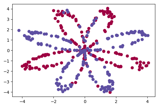
首先，我们导入需要工作的数据。下面的代码将导入一个 "flower"二分类数据集到变量 X 和 Y.

X, Y = load_planar_dataset()

使用matplotlib可视化数据集。数据看起来像一朵“花”，上面有一些红色(标签y=0)和一些蓝色(y=1)点。您的目标是建立一个适合这些数据的模型。 

# Visualize the data: c: 颜色；s:线宽； cmap：模块pyplot内置了一组颜色映射
plt.scatter(X[0, :], X[1, :], c=Y.reshape(400), s=40, cmap=plt.cm.Spectral);

你有：

• 一个 numpy-array （矩阵）X： 包含你的特征（x1, x2）
• 一个 numpy-array （向量）Y： 包含你的标签（red:0,  blue:1）.

来第一次得到更好的数据是什么样子的感觉：

 Exercise: 你有多少训练样本？另外，X和Y的维度是什么？

### START CODE HERE ### (≈ 3 lines of code)
shape_X = X.shape
shape_Y = Y.shape
m = shape_X[1]  # training set size
### END CODE HERE ###

print ('The shape of X is: ' + str(shape_X))
print ('The shape of Y is: ' + str(shape_Y))
print ('I have m = %d training examples!' % (m))

The shape of X is: (2, 400)
The shape of Y is: (1, 400)
I have m = 400 training examples!

Expected Output:

shape of X	(2, 400)
shape of Y	(1, 400)
m	400

3 - Simple Logistic Regression(简单的逻辑回归)

在建立一个完整的神经网络之前，让我们先看看逻辑回归在这个问题上的表现。可以使用sklearn的内置函数来实现这一点。运行下面的代码来训练数据集上的逻辑回归分类器。

# Train the logistic regression classifier
clf = sklearn.linear_model.LogisticRegressionCV();
clf.fit(X.T, Y.T);

3.1 绘制这些模型的决策边界

# Plot the decision boundary for logistic regression
plot_decision_boundary(lambda x: clf.predict(x), X, Y)
plt.title("Logistic Regression")

# Print accuracy
LR_predictions = clf.predict(X.T)
print ('Accuracy of logistic regression: %d ' % float((np.dot(Y,LR_predictions) + np.dot(1-Y,1-LR_predictions))/float(Y.size)*100) +
       '% ' + "(percentage of correctly labelled datapoints)")

Accuracy of logistic regression: 47 % (percentage of correctly labelled datapoints)

 解释:数据集不是线性可分的,所以逻辑回归不表现良好。希望一个神经网络能做得更好。现在让我们试试这个!

4 - Neural Network model（神经网络模型）

Logistic回归在“flower dataset”上效果不佳。你要训练一个只有一个隐藏层的神经网络

Here is our model:

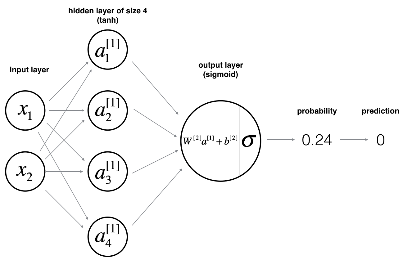
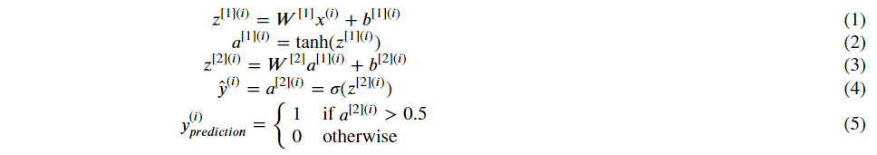
Mathematically:

For one example x(i):

提醒：建立神经网络的一般方法是：

1.  定义神经网络结构（神经网络的输入单元，隐藏单元，输出单元等）
2. 随机初始化模型的参数
3. 循环：

• • 实现前向传播
  • 计算损失值
  • 实现后向传播来获得梯度值
  • 更新参数（梯度下降）

  构建helper函数来计算步骤1-3，然后融合他们为一个 nn_model()函数。学习正确的参数，你可以在新数据上做出预测。

4.1 - Defining the neural network structure

Exercise: Define three variables:

• n_x: 输入层的大小
• n_h: 隐藏层的大小（设置为4）
• n_y: 输出层的大小

Hint: 使用X 和 Y 的维度来计算 n_x, n_y。隐藏层大小设置为4

# GRADED FUNCTION: layer_sizes

def layer_sizes(X, Y):
    """
    Arguments:
    X -- input dataset of shape (input size, number of examples)
    Y -- labels of shape (output size, number of examples)
    
    Returns:
    n_x -- the size of the input layer
    n_h -- the size of the hidden layer
    n_y -- the size of the output layer
    """
    ### START CODE HERE ### (≈ 3 lines of code)
    
    n_x = X.shape[0] # size of input layer
    n_h = 4
    n_y = Y.shape[0] # size of output layer
    
    ### END CODE HERE ###
    return (n_x, n_h, n_y)

X_assess, Y_assess = layer_sizes_test_case()
(n_x, n_h, n_y) = layer_sizes(X_assess, Y_assess)
print("The size of the input layer is: n_x = " + str(n_x))
print("The size of the hidden layer is: n_h = " + str(n_h))
print("The size of the output layer is: n_y = " + str(n_y))

The size of the input layer is: n_x = 5
The size of the hidden layer is: n_h = 4
The size of the output layer is: n_y = 2

Expected Output (these are not the sizes you will use for your network, they are just used to assess the function you've just coded).

n_x	5
n_h	4
n_y	2

4.2 - Initialize the model's parameters（初始化模型参数）

Exercise: Implement the function  initialize_parameters(). 

Instructions:

• 确认你的参数正确。
• 使用 随机值初始化权重矩阵。
  • 使用:  np.random.randn(a,b) * 0.01  来随机初始化(a, b)维度的矩阵。
• 把 偏置向量初始化为零。
  • 使用:  np.zeros((a,b))  用 0 初始化(a, b) 维度的矩阵

# GRADED FUNCTION: initialize_parameters

def initialize_parameters(n_x, n_h, n_y):
    """
    Argument:
    n_x -- size of the input layer
    n_h -- size of the hidden layer
    n_y -- size of the output layer
    
    Returns:
    params -- python dictionary containing your parameters:
                    W1 -- weight matrix of shape (n_h, n_x)
                    b1 -- bias vector of shape (n_h, 1)
                    W2 -- weight matrix of shape (n_y, n_h)
                    b2 -- bias vector of shape (n_y, 1)
    """
    
    np.random.seed(2) # we set up a seed so that your output matches ours although the initialization is random.
    
    ### START CODE HERE ### (≈ 4 lines of code)
    
    W1 = np.random.randn(n_h, n_x) * 0.01
    b1 = np.zeros(shape=(n_h, 1))
    W2 = np.random.randn(n_y, n_h) * 0.01
    b2 = np.zeros(shape=(n_y, 1))
    
    ### END CODE HERE ###
    
    assert (W1.shape == (n_h, n_x))
    assert (b1.shape == (n_h, 1))
    assert (W2.shape == (n_y, n_h))
    assert (b2.shape == (n_y, 1))
    
    parameters = {"W1": W1,
                  "b1": b1,
                  "W2": W2,
                  "b2": b2}
    
    return parameters

n_x, n_h, n_y = initialize_parameters_test_case()

parameters = initialize_parameters(n_x, n_h, n_y)

print("W1 = " + str(parameters["W1"]))
print("b1 = " + str(parameters["b1"]))
print("W2 = " + str(parameters["W2"]))
print("b2 = " + str(parameters["b2"]))

W1 = [[-0.00416758 -0.00056267]
 [-0.02136196  0.01640271]
 [-0.01793436 -0.00841747]
 [ 0.00502881 -0.01245288]]
b1 = [[ 0.]
 [ 0.]
 [ 0.]
 [ 0.]]
W2 = [[-0.01057952 -0.00909008  0.00551454  0.02292208]]
b2 = [[ 0.]]

Expected Output:

W1	[[-0.00416758 -0.00056267] [-0.02136196 0.01640271] [-0.01793436 -0.00841747] [ 0.00502881 -0.01245288]]
b1	[[ 0.] [ 0.] [ 0.] [ 0.]]
W2	[[-0.01057952 -0.00909008 0.00551454 0.02292208]]
b2	[[ 0.]]

4.3 - The Loop

Question: 实现前向传播 forward_propagation().

Instructions:

• 查看上面的数学公式表示你的分类器
• 使用  sigmoid() 
• 你可以使用 function  np.tanh() . 这是 numpy库的一部分
• 这些步骤你必须实现：

1. 从字典 "parameters" （initialize_parameters()的输出）检索每个参数，用 parameters["..."]。
2. 实现前向传播。计算： （所有训练集样本预测的向量）

• 反向传播所需的值存储在“cache”。cache将作为反向传播函数的输入。

# GRADED FUNCTION: forward_propagation

def forward_propagation(X, parameters):
    """
    Argument:
    X -- input data of size (n_x, m)
    parameters -- python dictionary containing your parameters (output of initialization function)
    
    Returns:
    A2 -- The sigmoid output of the second activation
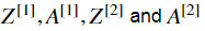
    cache -- a dictionary containing "Z1", "A1", "Z2" and "A2"
    """
    # Retrieve each parameter from the dictionary "parameters"
    ### START CODE HERE ### (≈ 4 lines of code)
    W1 = parameters["W1"]
    b1 = parameters["b1"]
    W2 = parameters["W2"]
    b2 = parameters["b2"]
    ### END CODE HERE ###
    
    # Implement Forward Propagation to calculate A2 (probabilities)
    ### START CODE HERE ### (≈ 4 lines of code)
    Z1 = np.dot(W1, X) + b1
    A1 = np.tanh(Z1)
    Z2 = np.dot(W2, A1) + b2 
    A2 = sigmoid(Z2)
    
#     print (W1.shape)
#     print (X.shape)
#     print (b1.shape)
#     print ("A1:", A1.shape)
#     print ("Z1:",Z1.shape)
#     print ("Z2:", Z2.shape)
#     print ("A2:", A2.shape)
    
    ### END CODE HERE ###
    
    assert(A2.shape == (1, X.shape[1]))
    
    cache = {"Z1": Z1,
             "A1": A1,
             "Z2": Z2,
             "A2": A2}
    
    return A2, cache

X_assess, parameters = forward_propagation_test_case()
A2, cache = forward_propagation(X_assess, parameters)

# Note: we use the mean here just to make sure that your output matches ours. 
print(np.mean(cache['Z1']) ,np.mean(cache['A1']),np.mean(cache['Z2']),np.mean(cache['A2']))

Expected Output:

0.262818640198 0.091999045227 -1.30766601287 0.212877681719

 现在你已经计算（在Python变量“A2”中），其中包含了每个示例的，你可以如下计算代价函数

Exercise: Implement  compute_cost()  to compute the value of the cost J.

Instructions:

• 实现交叉熵损失（cross-entropy loss）的方法有很多种。我们如何实现

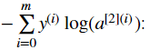
logprobs = np.multiply(np.log(A2),Y)
cost = - np.sum(logprobs)                # no need to use a for loop!

# GRADED FUNCTION: compute_cost

def compute_cost(A2, Y, parameters):
    """
    Computes the cross-entropy cost given in equation (13)
    
    Arguments:
    A2 -- The sigmoid output of the second activation, of shape (1, number of examples)
    Y -- "true" labels vector of shape (1, number of examples)
    parameters -- python dictionary containing your parameters W1, b1, W2 and b2
    
    Returns:
    cost -- cross-entropy cost given equation (13)
    """
    
    m = Y.shape[1] # number of example

    # Compute the cross-entropy cost
    ### START CODE HERE ### (≈ 2 lines of code)
    logprobs = np.multiply(np.log(A2), Y) + np.multiply(np.log(1 - A2), 1 - Y)
    cost = - np.sum(logprobs) / m
    ### END CODE HERE ###
    
    cost = np.squeeze(cost)     # makes sure cost is the dimension we expect. 
                                # E.g., turns [[17]] into 17 
    assert(isinstance(cost, float))
    
    return cost

A2, Y_assess, parameters = compute_cost_test_case()

print("cost = " + str(compute_cost(A2, Y_assess, parameters)))

cost = 0.692919893776

Expected Output:

cost	0.693058761...

使用前向传播期间的cache, 现在可以实现反向传播。

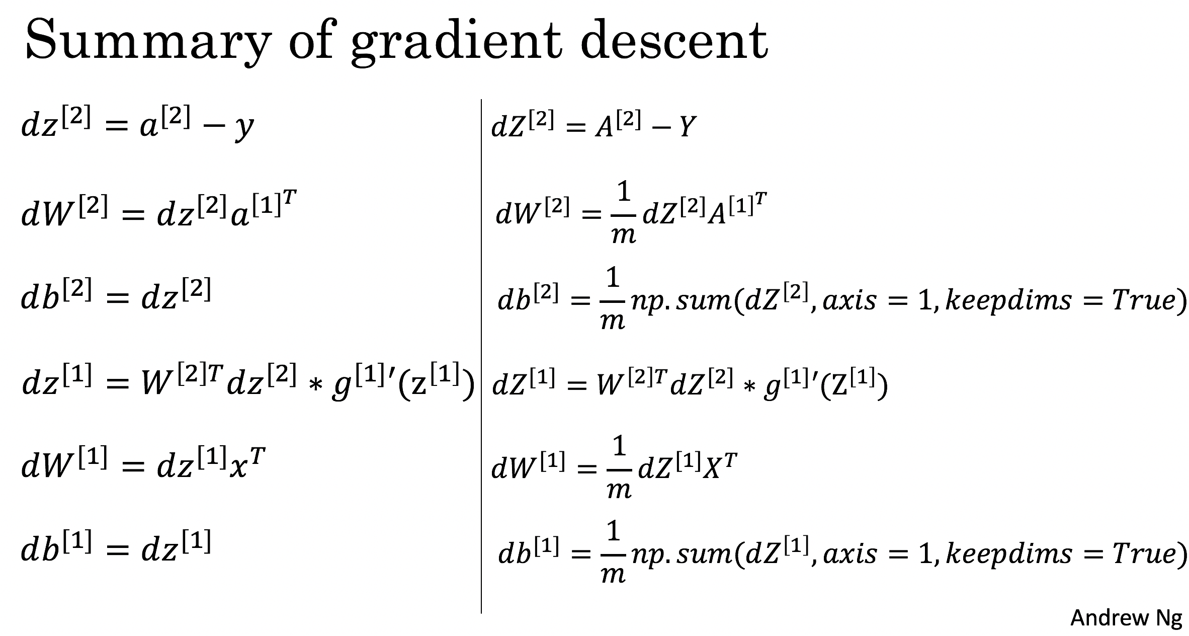
Question: Implement the function  backward_propagation(). 

Instructions: 下面提供6个公式矢量化的实现。

Tips: 

计算 dZ1，你需要计算 。由于是一个 tanh 激励函数，如果 

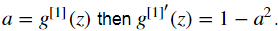
所以你可以用(1 - np.power(A1, 2)) 计算 。

# GRADED FUNCTION: backward_propagation

def backward_propagation(parameters, cache, X, Y):
    """
    Implement the backward propagation using the instructions above.
    
    Arguments:
    parameters -- python dictionary containing our parameters 
    cache -- a dictionary containing "Z1", "A1", "Z2" and "A2".
    X -- input data of shape (2, number of examples)
    Y -- "true" labels vector of shape (1, number of examples)
    
    Returns:
    grads -- python dictionary containing your gradients with respect to different parameters
    """
    m = X.shape[1]
    
    # First, retrieve W1 and W2 from the dictionary "parameters".
    ### START CODE HERE ### (≈ 2 lines of code)
    W1 = parameters["W1"]
    W2 = parameters["W2"]
    ### END CODE HERE ###
        
    # Retrieve also A1 and A2 from dictionary "cache".
    ### START CODE HERE ### (≈ 2 lines of code)
    A1 = cache["A1"]
    A2 = cache["A2"]
    ### END CODE HERE ###
    
    # Backward propagation: calculate dW1, db1, dW2, db2. 
    ### START CODE HERE ### (≈ 6 lines of code, corresponding to 6 equations on slide above)
    dZ2 = A2 - Y
    dW2 = (1 / m) * np.dot(dZ2, A1.T)
    db2 = (1 / m) * np.sum(dZ2, axis=1, keepdims=True)
    dZ1 = np.multiply(np.dot(W2.T, dZ2), 1 - np.power(A1, 2))
    dW1 = (1 / m) * np.dot(dZ1, X.T)
    db1 = (1 / m) * np.sum(dZ1, axis=1, keepdims=True) 
    ### END CODE HERE ###
    
    grads = {"dW1": dW1,
             "db1": db1,
             "dW2": dW2,
             "db2": db2}
    
    return grads

parameters, cache, X_assess, Y_assess = backward_propagation_test_case()

grads = backward_propagation(parameters, cache, X_assess, Y_assess)
print ("dW1 = "+ str(grads["dW1"]))
print ("db1 = "+ str(grads["db1"]))
print ("dW2 = "+ str(grads["dW2"]))
print ("db2 = "+ str(grads["db2"]))

dW1 = [[ 0.01018708 -0.00708701]
 [ 0.00873447 -0.0060768 ]
 [-0.00530847  0.00369379]
 [-0.02206365  0.01535126]]
db1 = [[-0.00069728]
 [-0.00060606]
 [ 0.000364  ]
 [ 0.00151207]]
dW2 = [[ 0.00363613  0.03153604  0.01162914 -0.01318316]]
db2 = [[ 0.06589489]]

Expected output:

dW1	[[ 0.01018708 -0.00708701] [ 0.00873447 -0.0060768 ] [-0.00530847 0.00369379] [-0.02206365 0.01535126]]
db1	[[-0.00069728] [-0.00060606] [ 0.000364 ] [ 0.00151207]]
dW2	[[ 0.00363613 0.03153604 0.01162914 -0.01318316]]
db2	[[ 0.06589489]]

Question: 执行更新参数规则。使用梯度下降算法。你不得不使用 (dW1, db1, dW2, db2) 来更新 (W1, b1, W2, b2).

一般梯度下降规则：。（α 是learning rate；θ 表示参数）

Illustration: 梯度下降算法具有良好的学习速率（收敛） 和 差的学习速率（发散）。图片如下：.

# GRADED FUNCTION: update_parameters

def update_parameters(parameters, grads, learning_rate = 1.2):
    """
    Updates parameters using the gradient descent update rule given above
    
    Arguments:
    parameters -- python dictionary containing your parameters 
    grads -- python dictionary containing your gradients 
    
    Returns:
    parameters -- python dictionary containing your updated parameters 
    """
    # Retrieve each parameter from the dictionary "parameters"
    ### START CODE HERE ### (≈ 4 lines of code)
    W1 = parameters["W1"]
    b1 = parameters["b1"]
    W2 = parameters["W2"]
    b2 = parameters["b2"]
    ### END CODE HERE ###
    
    # Retrieve each gradient from the dictionary "grads"
    ### START CODE HERE ### (≈ 4 lines of code)
    dW1 = grads["dW1"]
    db1 = grads["db1"]
    dW2 = grads["dW2"]
    db2 = grads["db2"]
    ## END CODE HERE ###
    
    # Update rule for each parameter
    ### START CODE HERE ### (≈ 4 lines of code)
    W1 = W1 - learning_rate * dW1
    b1 = b1 - learning_rate * db1
    W2 = W2 - learning_rate * dW2
    b2 = b2 - learning_rate * db2
    ### END CODE HERE ###
    
    parameters = {"W1": W1,
                  "b1": b1,
                  "W2": W2,
                  "b2": b2}
    
    return parameters

parameters, grads = update_parameters_test_case()
parameters = update_parameters(parameters, grads)

print("W1 = " + str(parameters["W1"]))
print("b1 = " + str(parameters["b1"]))
print("W2 = " + str(parameters["W2"]))
print("b2 = " + str(parameters["b2"]))

W1 = [[-0.00643025  0.01936718]
 [-0.02410458  0.03978052]
 [-0.01653973 -0.02096177]
 [ 0.01046864 -0.05990141]]
b1 = [[ -1.02420756e-06]
 [  1.27373948e-05]
 [  8.32996807e-07]
 [ -3.20136836e-06]]
W2 = [[-0.01041081 -0.04463285  0.01758031  0.04747113]]
b2 = [[ 0.00010457]]

Expected Output:

W1	[[-0.00643025 0.01936718] [-0.02410458 0.03978052] [-0.01653973 -0.02096177] [ 0.01046864 -0.05990141]]
b1	[[ -1.02420756e-06] [ 1.27373948e-05] [ 8.32996807e-07] [ -3.20136836e-06]]
W2	[[-0.01041081 -0.04463285 0.01758031 0.04747113]]
b2	[[ 0.00010457]]

4.4 - Integrate parts 4.1, 4.2 and 4.3 in nn_model()

Question: 在 nn_model() 里构建神经网络模型

Instructions: 神经网络模型必须按照正确的顺序使用前面的函数。

# GRADED FUNCTION: nn_model

def nn_model(X, Y, n_h, num_iterations=10000, print_cost=False):
    """
    Arguments:
    X -- dataset of shape (2, number of examples)
    Y -- labels of shape (1, number of examples)
    n_h -- size of the hidden layer
    num_iterations -- Number of iterations in gradient descent loop
    print_cost -- if True, print the cost every 1000 iterations
    
    Returns:
    parameters -- parameters learnt by the model. They can then be used to predict.
    """
    
    np.random.seed(3)
    n_x = layer_sizes(X, Y)[0]
    n_y = layer_sizes(X, Y)[2]
    
    # Initialize parameters, then retrieve W1, b1, W2, b2. Inputs: "n_x, n_h, n_y". Outputs = "W1, b1, W2, b2, parameters".
    ### START CODE HERE ### (≈ 5 lines of code)
    parameters = initialize_parameters(n_x, n_h, n_y)
    W1 = parameters['W1']
    b1 = parameters['b1']
    W2 = parameters['W2']
    b2 = parameters['b2']
    ### END CODE HERE ###
    
    # Loop (gradient descent)

    for i in range(0, num_iterations):
         
        ### START CODE HERE ### (≈ 4 lines of code)
        # Forward propagation. Inputs: "X, parameters". Outputs: "A2, cache".
        A2, cache = forward_propagation(X, parameters)
        
        # Cost function. Inputs: "A2, Y, parameters". Outputs: "cost".
        cost = compute_cost(A2, Y, parameters)
 
        # Backpropagation. Inputs: "parameters, cache, X, Y". Outputs: "grads".
        grads = backward_propagation(parameters, cache, X, Y)
 
        # Gradient descent parameter update. Inputs: "parameters, grads". Outputs: "parameters".
        parameters = update_parameters(parameters, grads)
        
        ### END CODE HERE ###
        
        # Print the cost every 1000 iterations
        if print_cost and i % 1000 == 0:
            print ("Cost after iteration %i: %f" % (i, cost))

    return parameters

X_assess, Y_assess = nn_model_test_case()

parameters = nn_model(X_assess, Y_assess, 4, num_iterations=10000, print_cost=True)
print("W1 = " + str(parameters["W1"]))
print("b1 = " + str(parameters["b1"]))
print("W2 = " + str(parameters["W2"]))
print("b2 = " + str(parameters["b2"]))

Expected Output:

W1	[[-4.18494056 5.33220609] [-7.52989382 1.24306181] [-4.1929459 5.32632331] [ 7.52983719 -1.24309422]]
b1	[[ 2.32926819] [ 3.79458998] [ 2.33002577] [-3.79468846]]
W2	[[-6033.83672146 -6008.12980822 -6033.10095287 6008.06637269]]
b2	[[-52.66607724]]

4.5 - Predictions

Question: 使用您的模型通过构建 predict()来进行预测。使用前向传播来预测结果。.

Reminder:

 

 

例如，如果要根据阈值将 matrix X 条目设置为 0 和 1，则需要执行以下操作： X_new = (X > threshold)

# GRADED FUNCTION: predict

def predict(parameters, X):
    """
    Using the learned parameters, predicts a class for each example in X
    
    Arguments:
    parameters -- python dictionary containing your parameters 
    X -- input data of size (n_x, m)
    
    Returns
    predictions -- vector of predictions of our model (red: 0 / blue: 1)
    """
    
    # Computes probabilities using forward propagation, and classifies to 0/1 using 0.5 as the threshold.
    ### START CODE HERE ### (≈ 2 lines of code)
    A2, cache = forward_propagation(X, parameters)
    predictions = np.round(A2)
    ### END CODE HERE ###
    
    return predictions

parameters, X_assess = predict_test_case()

predictions = predict(parameters, X_assess)
print("predictions mean = " + str(np.mean(predictions)))

Expected Output:

predictions mean

0.666666666667

 使用单个隐藏层，n_h个隐藏单元测试模型。

# Build a model with a n_h-dimensional hidden layer
parameters = nn_model(X, Y, n_h = 4, num_iterations = 10000, print_cost=True)

# Plot the decision boundary
plot_decision_boundary(lambda x: predict(parameters, x.T), X, Y)
plt.title("Decision Boundary for hidden layer size " + str(4))

Cost after iteration 0: 0.693048
Cost after iteration 1000: 0.288083
Cost after iteration 2000: 0.254385
Cost after iteration 3000: 0.233864
Cost after iteration 4000: 0.226792
Cost after iteration 5000: 0.222644
Cost after iteration 6000: 0.219731
Cost after iteration 7000: 0.217504
Cost after iteration 8000: 0.219440
Cost after iteration 9000: 0.218553

Expected Output:

Cost after iteration 9000

0.218607

 

# Print accuracy
predictions = predict(parameters, X)
print ('Accuracy: %d' % float((np.dot(Y,predictions.T) + np.dot(1-Y,1-predictions.T))/float(Y.size)*100) + '%')

Expected Output:

Accuracy

90%

 与Logistic回归相比，准确性很高。这个模型已经学会了花的叶子图案！与Logistic回归不同，神经网络甚至能够学习高度非线性的决策边界.现在，让我们尝试几个隐藏层的大小。

4.6 - Tuning hidden layer size (optional/ungraded exercise)（调整隐藏层大小）

您将观察不同隐藏层大小的模型的不同行为。

# This may take about 2 minutes to run

plt.figure(figsize=(16, 32))  # 设置图像大小
hidden_layer_sizes = [1, 2, 3, 4, 5, 20, 50]
for i, n_h in enumerate(hidden_layer_sizes):
    plt.subplot(5, 2, i+1)
    plt.title('Hidden Layer of size %d' % n_h)
    parameters = nn_model(X, Y, n_h, num_iterations = 5000)
    plot_decision_boundary(lambda x: predict(parameters, x.T), X, Y)
    predictions = predict(parameters, X)
    accuracy = float((np.dot(Y,predictions.T) + np.dot(1-Y,1-predictions.T))/float(Y.size)*100)
    print ("Accuracy for {} hidden units: {} %".format(n_h, accuracy))

Accuracy for 1 hidden units: 67.5 %
Accuracy for 2 hidden units: 67.25 %
Accuracy for 3 hidden units: 90.75 %
Accuracy for 4 hidden units: 90.5 %
Accuracy for 5 hidden units: 91.25 %
Accuracy for 20 hidden units: 90.5 %
Accuracy for 50 hidden units: 90.75 %

 

Interpretation:

• 较大的模型（有更多的隐藏单元）能够更好地适应训练集。直到最终最大的模型过拟合数据。
• 最好的隐藏层大小似乎在n_h=5左右。实际上，这里似乎与数据很好的吻合。同时也不好引起明显的过拟合。
• 稍后你还能了解正则化（regularization），他允许你使用非常大的模型（例如n_h = 50），而且没有太多过拟合。

Optional questions:

• 可以将tanh激活函数改成 sigmoid() 和 relu 激活函数时，会发生什么？
• 修改学习率（learning rate）
• 如果更改数据集怎么办？

你已经学会了：

• 建立一个完整的隐藏神经网络
• 充分利用一个非线性单元实现前向传播和反向传播，并训练一个神经网络
• 看看改变隐层大小的影响，包括过拟合。

5 - Performance on other datasets

如果需要，可以为下列每个数据集重新运行整个notebook(减去DataSet部分)。

# Datasets
noisy_circles, noisy_moons, blobs, gaussian_quantiles, no_structure = load_extra_datasets()

datasets = {"noisy_circles": noisy_circles,
            "noisy_moons": noisy_moons,
            "blobs": blobs,
            "gaussian_quantiles": gaussian_quantiles}

### START CODE HERE ### (choose your dataset)
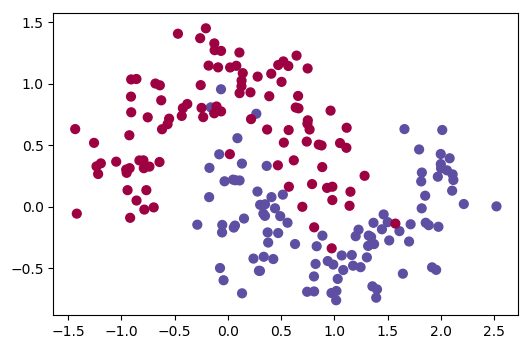
dataset = "noisy_moons"
### END CODE HERE ###

X, Y = datasets[dataset]
X, Y = X.T, Y.reshape(1, Y.shape[0])

# make blobs binary
if dataset == "blobs":
    Y = Y % 2

# Visualize the data
plt.scatter(X[0, :], X[1, :], c=Y.reshape(200), s=40, cmap=plt.cm.Spectral);

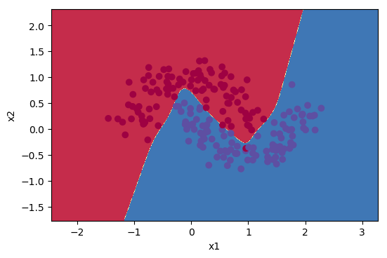
parameters = nn_model(X, Y, n_h=5, num_iterations = 5000)
plot_decision_boundary(lambda x: predict(parameters, x.T), X, Y)

predictions = predict(parameters, X)
accuracy = float((np.dot(Y,predictions.T) + np.dot(1-Y,1-predictions.T))/float(Y.size)*100)
print("Accuracy: ", accuracy)