记录一下faster rcnn

http://www.telesens.co/2018/03/11/object-detection-and-classification-using-r-cnns/

经过R-CNN和Fast RCNN的积淀，Ross B. Girshick在2016年提出了新的Faster RCNN，在结构上，Faster RCNN已经将特征抽取(feature extraction)，proposal提取，bounding box regression(rect refine)，classification都整合在了一个网络中，使得综合性能有较大提高，在检测速度方面尤为明显。

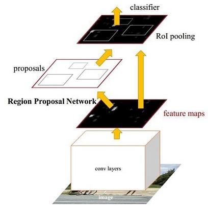图1 Faster RCNN基本结构（来自原论文）

依作者看来，如图1，Faster RCNN其实可以分为4个主要内容：

Conv layers。作为一种CNN网络目标检测方法，Faster RCNN首先使用一组基础的conv+relu+pooling层提取image的feature maps。该feature maps被共享用于后续RPN层和全连接层。
Region Proposal Networks。RPN网络用于生成region proposals。该层通过softmax判断anchors属于foreground或者background，再利用bounding box regression修正anchors获得精确的proposals。
Roi Pooling。该层收集输入的feature maps和proposals，综合这些信息后提取proposal feature maps，送入后续全连接层判定目标类别。
Classification。利用proposal feature maps计算proposal的类别，同时再次bounding box regression获得检测框最终的精确位置。

所以本文以上述4个内容作为切入点介绍Faster R-CNN网络。
图2展示了python版本中的VGG16模型中的faster_rcnn_test.pt的网络结构，可以清晰的看到该网络对于一副任意大小PxQ的图像，首先缩放至固定大小MxN，然后将MxN图像送入网络；而Conv layers中包含了13个conv层+13个relu层+4个pooling层；RPN网络首先经过3x3卷积，再分别生成foreground anchors与bounding box regression偏移量，然后计算出proposals；而Roi Pooling层则利用proposals从feature maps中提取proposal feature送入后续全连接和softmax网络作classification（即分类proposal到底是什么object）。

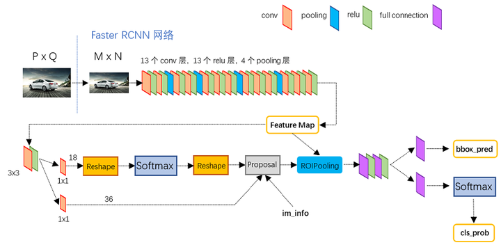图2 faster_rcnn_test.pt网络结构（pascal_voc/VGG16/faster_rcnn_alt_opt/faster_rcnn_test.pt）

本文不会讨论任何关于R-CNN家族的历史，分析清楚最新的Faster R-CNN就够了，并不需要追溯到那么久。实话说我也不了解R-CNN，更不关心。有空不如看看新算法。

1 Conv layers

Conv layers包含了conv，pooling，relu三种层。以python版本中的VGG16模型中的faster_rcnn_test.pt的网络结构为例，如图2，Conv layers部分共有13个conv层，13个relu层，4个pooling层。这里有一个非常容易被忽略但是又无比重要的信息，在Conv layers中：

所有的conv层都是： $kernel\_size=3$ ， $pad=1$ ， $stride=1$
所有的pooling层都是： $kernel\_size=2$ ， $pad=0$ ， $stride=2$

为何重要？在Faster RCNN Conv layers中对所有的卷积都做了扩边处理（ pad=1，即填充一圈0），导致原图变为 (M+2)x(N+2)大小，再做3x3卷积后输出MxN 。正是这种设置，导致Conv layers中的conv层不改变输入和输出矩阵大小。如图3：

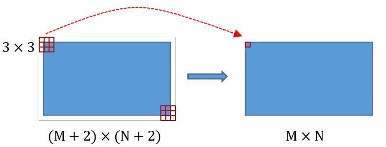图3 卷积示意图

类似的是，Conv layers中的pooling层kernel_size=2，stride=2。这样每个经过pooling层的MxN矩阵，都会变为(M/2)x(N/2)大小。综上所述，在整个Conv layers中，conv和relu层不改变输入输出大小，只有pooling层使输出长宽都变为输入的1/2。
那么，一个MxN大小的矩阵经过Conv layers固定变为(M/16)x(N/16)！这样Conv layers生成的featuure map中都可以和原图对应起来。

2 Region Proposal Networks(RPN)

经典的检测方法生成检测框都非常耗时，如OpenCV adaboost使用滑动窗口+图像金字塔生成检测框；或如R-CNN使用SS(Selective Search)方法生成检测框。而Faster RCNN则抛弃了传统的滑动窗口和SS方法，直接使用RPN生成检测框，这也是Faster R-CNN的巨大优势，能极大提升检测框的生成速度。

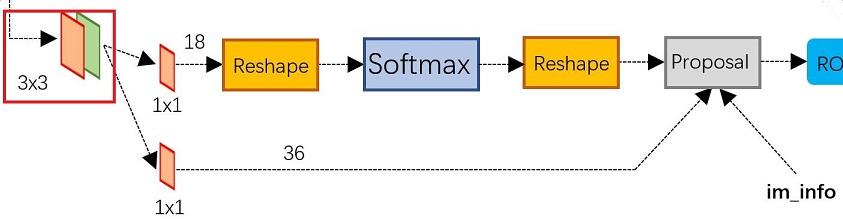图4 RPN网络结构

上图4展示了RPN网络的具体结构。可以看到RPN网络实际分为2条线，上面一条通过softmax分类anchors获得foreground和background（检测目标是foreground），下面一条用于计算对于anchors的bounding box regression偏移量，以获得精确的proposal。而最后的Proposal层则负责综合foreground anchors和bounding box regression偏移量获取proposals，同时剔除太小和超出边界的proposals。其实整个网络到了Proposal Layer这里，就完成了相当于目标定位的功能。

2.1 多通道图像卷积基础知识介绍

在介绍RPN前，还要多解释几句基础知识，已经懂的看官老爷跳过就好。

对于单通道图像+单卷积核做卷积，第一章中的图3已经展示了；
对于多通道图像+多卷积核做卷积，计算方式如下：

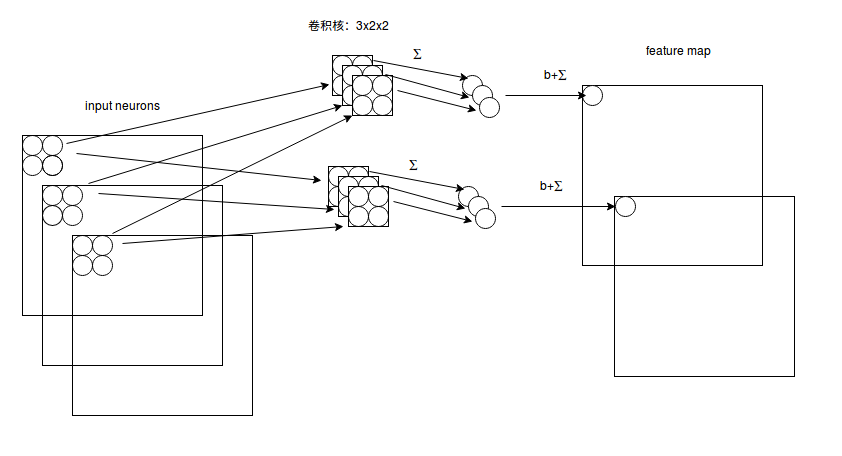图5 多通道卷积计算方式

如图5，输入有3个通道，同时有2个卷积核。对于每个卷积核，先在输入3个通道分别作卷积，再将3个通道结果加起来得到卷积输出。所以对于某个卷积层，无论输入图像有多少个通道，输出图像通道数总是等于卷积核数量！
对多通道图像做1x1卷积，其实就是将输入图像于每个通道乘以卷积系数后加在一起，即相当于把原图像中本来各个独立的通道“联通”在了一起。

2.2 anchors

提到RPN网络，就不能不说anchors。所谓anchors，实际上就是一组由rpn/generate_anchors.py生成的矩形。直接运行作者demo中的generate_anchors.py可以得到以下输出：

[[ -84.  -40.   99.   55.]
 [-176.  -88.  191.  103.]
 [-360. -184.  375.  199.]
 [ -56.  -56.   71.   71.]
 [-120. -120.  135.  135.]
 [-248. -248.  263.  263.]
 [ -36.  -80.   51.   95.]
 [ -80. -168.   95.  183.]
 [-168. -344.  183.  359.]]

其中每行的4个值(x1, y1, x2, y2) 表矩形左上和右下角点坐标。9个矩形共有3种形状，长宽比为大约为with:height∈{1:1, 1:2, 2:1}三种，如图6。实际上通过anchors就引入了检测中常用到的多尺度方法。

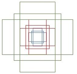图6 anchors示意图

注：关于上面的anchors size，其实是根据检测图像设置的。在python demo中，会把任意大小的输入图像reshape成800x600（即图2中的M=800，N=600）。再回头来看anchors的大小，anchors中长宽1:2中最大为352x704，长宽2:1中最大736x384，基本是cover了800x600的各个尺度和形状。
那么这9个anchors是做什么的呢？借用Faster RCNN论文中的原图，如图7，遍历Conv layers计算获得的feature maps，为每一个点都配备这9种anchors作为初始的检测框。这样做获得检测框很不准确，不用担心，后面还有2次bounding box regression可以修正检测框位置。

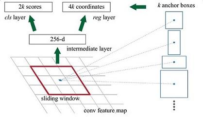图7

解释一下上面这张图的数字。

在原文中使用的是ZF model中，其Conv Layers中最后的conv5层num_output=256，对应生成256张特征图，所以相当于feature map每个点都是256-dimensions
在conv5之后，做了rpn_conv/3x3卷积且num_output=256，相当于每个点又融合了周围3x3的空间信息（猜测这样做也许更鲁棒？反正我没测试），同时256-d不变（如图4和图7中的红框）
假设在conv5 feature map中每个点上有k个anchor（默认k=9），而每个anhcor要分foreground和background，所以每个点由256d feature转化为cls=2k scores；而每个anchor都有[x, y, w, h]对应4个偏移量，所以reg=4k coordinates
补充一点，全部anchors拿去训练太多了，训练程序会在合适的anchors中随机选取128个postive anchors+128个negative anchors进行训练（什么是合适的anchors下文5.1有解释）

注意，在本文讲解中使用的VGG conv5 num_output=512，所以是512d，其他类似。

其实RPN最终就是在原图尺度上，设置了密密麻麻的候选Anchor。然后用cnn去判断哪些Anchor是里面有目标的foreground anchor，哪些是没目标的backgroud。所以，仅仅是个二分类而已！

那么Anchor一共有多少个？原图800x600，VGG下采样16倍，feature map每个点设置9个Anchor，所以：

$ceil(800/16) \times ceil(600/16) \times 9=50\times38 \times9=17100$

其中ceil()表示向上取整，是因为VGG输出的feature map size= 50*38。

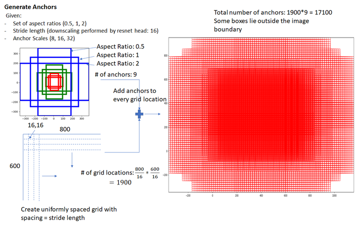图8 Gernerate Anchors

看官老爷们，这还不懂？再问Anchor怎么来的直播跳楼！

2.3 softmax判定foreground与background

一副MxN大小的矩阵送入Faster RCNN网络后，到RPN网络变为(M/16)x(N/16)，不妨设 W=M/16，H=N/16。在进入reshape与softmax之前，先做了1x1卷积，如图9：

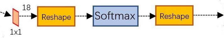图9 RPN中判定fg/bg网络结构

该1x1卷积的caffe prototxt定义如下：

layer {
  name: "rpn_cls_score"
  type: "Convolution"
  bottom: "rpn/output"
  top: "rpn_cls_score"
  convolution_param {
    num_output: 18   # 2(bg/fg) * 9(anchors)
    kernel_size: 1 pad: 0 stride: 1
  }
}

可以看到其num_output=18，也就是经过该卷积的输出图像为WxHx18大小（注意第二章开头提到的卷积计算方式）。这也就刚好对应了feature maps每一个点都有9个anchors，同时每个anchors又有可能是foreground和background，所有这些信息都保存WxHx(9*2)大小的矩阵。为何这样做？后面接softmax分类获得foreground anchors，也就相当于初步提取了检测目标候选区域box（一般认为目标在foreground anchors中）。
那么为何要在softmax前后都接一个reshape layer？其实只是为了便于softmax分类，至于具体原因这就要从caffe的实现形式说起了。在caffe基本数据结构blob中以如下形式保存数据：

blob=[batch_size, channel，height，width]

对应至上面的保存bg/fg anchors的矩阵，其在caffe blob中的存储形式为[1, 2x9, H, W]。而在softmax分类时需要进行fg/bg二分类，所以reshape layer会将其变为[1, 2, 9xH, W]大小，即单独“腾空”出来一个维度以便softmax分类，之后再reshape回复原状。贴一段caffe softmax_loss_layer.cpp的reshape函数的解释，非常精辟：

"Number of labels must match number of predictions; "
"e.g., if softmax axis == 1 and prediction shape is (N, C, H, W), "
"label count (number of labels) must be N*H*W, "
"with integer values in {0, 1, ..., C-1}.";

综上所述，RPN网络中利用anchors和softmax初步提取出foreground anchors作为候选区域。

2.4 bounding box regression原理

如图9所示绿色框为飞机的Ground Truth(GT)，红色为提取的foreground anchors，即便红色的框被分类器识别为飞机，但是由于红色的框定位不准，这张图相当于没有正确的检测出飞机。所以我们希望采用一种方法对红色的框进行微调，使得foreground anchors和GT更加接近。

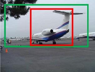图10

对于窗口一般使用四维向量 (x, y, w, h)表示，分别表示窗口的中心点坐标和宽高。对于图 11，红色的框A代表原始的Foreground Anchors，绿色的框G代表目标的GT，我们的目标是寻找一种关系，使得输入原始的anchor A经过映射得到一个跟真实窗口G更接近的回归窗口G'，即：

给定：anchor $A=(A_{x}, A_{y}, A_{w}, A_{h})$ 和 $GT=[G_{x}, G_{y}, G_{w}, G_{h}]$
寻找一种变换F，使得： $F(A_{x}, A_{y}, A_{w}, A_{h})=(G_{x}^{'}, G_{y}^{'}, G_{w}^{'}, G_{h}^{'})$ ，其中 $(G_{x}^{'}, G_{y}^{'}, G_{w}^{'}, G_{h}^{'})≈(G_{x}, G_{y}, G_{w}, G_{h})$

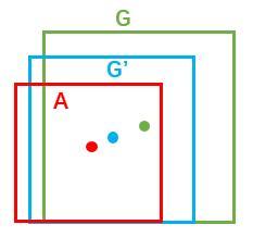图11

那么经过何种变换F才能从图10中的anchor A变为G'呢？比较简单的思路就是:

先做平移

再做缩放

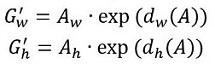
观察上面4个公式发现，需要学习的是 $d_{x}(A),d_{y}(A),d_{w}(A),d_{h}(A)$ 这四个变换。当输入的anchor A与GT相差较小时，可以认为这种变换是一种线性变换，那么就可以用线性回归来建模对窗口进行微调（注意，只有当anchors A和GT比较接近时，才能使用线性回归模型，否则就是复杂的非线性问题了）。
接下来的问题就是如何通过线性回归获得 $d_{x}(A),d_{y}(A),d_{w}(A),d_{h}(A)$ 了。线性回归就是给定输入的特征向量X, 学习一组参数W, 使得经过线性回归后的值跟真实值Y非常接近，即 $Y=WX$ 。对于该问题，输入X是cnn feature map，定义为Φ；同时还有训练传入A与GT之间的变换量，即 $(t_{x}, t_{y}, t_{w}, t_{h})$ 。输出是 $d_{x}(A),d_{y}(A),d_{w}(A),d_{h}(A)$ 四个变换。那么目标函数可以表示为：

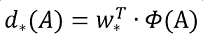
其中Φ(A)是对应anchor的feature map组成的特征向量，w是需要学习的参数，d(A)是得到的预测值（*表示 x，y，w，h，也就是每一个变换对应一个上述目标函数）。为了让预测值 $(t_{x}, t_{y}, t_{w}, t_{h})$ 与真实值差距最小，设计损失函数：

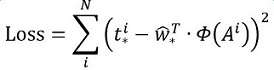
函数优化目标为：

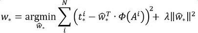
需要说明，只有在GT与需要回归框位置比较接近时，才可近似认为上述线性变换成立。
说完原理，对应于Faster RCNN原文，foreground anchor与ground truth之间的平移量 $(t_x, t_y)$ 与尺度因子 $(t_w, t_h)$ 如下：

对于训练bouding box regression网络回归分支，输入是cnn feature Φ，监督信号是Anchor与GT的差距 $(t_x, t_y, t_w, t_h)$ ，即训练目标是：输入 Φ的情况下使网络输出与监督信号尽可能接近。
那么当bouding box regression工作时，再输入Φ时，回归网络分支的输出就是每个Anchor的平移量和变换尺度 $(t_x, t_y, t_w, t_h)$ ，显然即可用来修正Anchor位置了。

2.5 对proposals进行bounding box regression

在了解bounding box regression后，再回头来看RPN网络第二条线路，如图12。

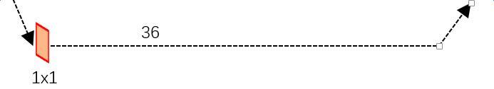图12 RPN中的bbox reg

先来看一看上图11中1x1卷积的caffe prototxt定义：

layer {
  name: "rpn_bbox_pred"
  type: "Convolution"
  bottom: "rpn/output"
  top: "rpn_bbox_pred"
  convolution_param {
    num_output: 36   # 4 * 9(anchors)
    kernel_size: 1 pad: 0 stride: 1
  }
}

可以看到其 num_output=36，即经过该卷积输出图像为WxHx36，在caffe blob存储为[1, 4x9, H, W]，这里相当于feature maps每个点都有9个anchors，每个anchors又都有4个用于回归的 $[d_{x}(A),d_{y}(A),d_{w}(A),d_{h}(A)]$ 变换量。

2.6 Proposal Layer

Proposal Layer负责综合所有 $[d_{x}(A),d_{y}(A),d_{w}(A),d_{h}(A)]$ 变换量和foreground anchors，计算出精准的proposal，送入后续RoI Pooling Layer。还是先来看看Proposal Layer的caffe prototxt定义：

layer {
  name: 'proposal'
  type: 'Python'
  bottom: 'rpn_cls_prob_reshape'
  bottom: 'rpn_bbox_pred'
  bottom: 'im_info'
  top: 'rois'
  python_param {
    module: 'rpn.proposal_layer'
    layer: 'ProposalLayer'
    param_str: "'feat_stride': 16"
  }
}

Proposal Layer有3个输入：fg/bg anchors分类器结果rpn_cls_prob_reshape，对应的bbox reg的 $[d_{x}(A),d_{y}(A),d_{w}(A),d_{h}(A)]$ 变换量rpn_bbox_pred，以及im_info；另外还有参数feat_stride=16，这和图4是对应的。
首先解释im_info。对于一副任意大小PxQ图像，传入Faster RCNN前首先reshape到固定MxN，im_info=[M, N, scale_factor]则保存了此次缩放的所有信息。然后经过Conv Layers，经过4次pooling变为WxH=(M/16)x(N/16)大小，其中feature_stride=16则保存了该信息，用于计算anchor偏移量。

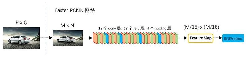图13

Proposal Layer forward（caffe layer的前传函数）按照以下顺序依次处理：

生成anchors，利用 $[d_{x}(A),d_{y}(A),d_{w}(A),d_{h}(A)]$ 对所有的anchors做bbox regression回归（这里的anchors生成和训练时完全一致）
按照输入的foreground softmax scores由大到小排序anchors，提取前pre_nms_topN(e.g. 6000)个anchors，即提取修正位置后的foreground anchors。
限定超出图像边界的foreground anchors为图像边界（防止后续roi pooling时proposal超出图像边界）
剔除非常小（width<threshold or height<threshold）的foreground anchors
进行nonmaximum suppression
再次按照nms后的foreground softmax scores由大到小排序fg anchors，提取前post_nms_topN(e.g. 300)结果作为proposal输出。

之后输出proposal=[x1, y1, x2, y2]，注意，由于在第三步中将anchors映射回原图判断是否超出边界，所以这里输出的proposal是对应MxN输入图像尺度的，这点在后续网络中有用。另外我认为，严格意义上的检测应该到此就结束了，后续部分应该属于识别了~
RPN网络结构就介绍到这里，总结起来就是：
生成anchors -> softmax分类器提取fg anchors -> bbox reg回归fg anchors -> Proposal Layer生成proposals

3 RoI pooling

而RoI Pooling层则负责收集proposal，并计算出proposal feature maps，送入后续网络。从图2中可以看到Rol pooling层有2个输入：

原始的feature maps
RPN输出的proposal boxes（大小各不相同）

3.1 为何需要RoI Pooling

先来看一个问题：对于传统的CNN（如AlexNet，VGG），当网络训练好后输入的图像尺寸必须是固定值，同时网络输出也是固定大小的vector or matrix。如果输入图像大小不定，这个问题就变得比较麻烦。有2种解决办法：

从图像中crop一部分传入网络
将图像warp成需要的大小后传入网络

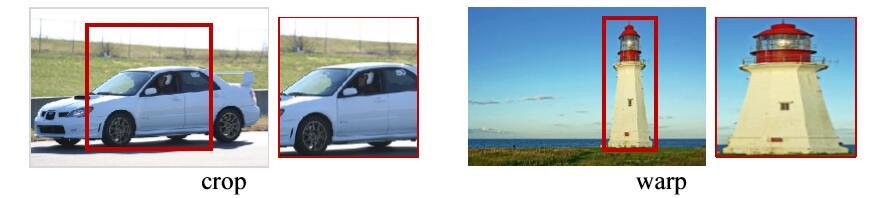图14 crop与warp破坏图像原有结构信息

两种办法的示意图如图14，可以看到无论采取那种办法都不好，要么crop后破坏了图像的完整结构，要么warp破坏了图像原始形状信息。
回忆RPN网络生成的proposals的方法：对foreground anchors进行bounding box regression，那么这样获得的proposals也是大小形状各不相同，即也存在上述问题。所以Faster R-CNN中提出了RoI Pooling解决这个问题。不过RoI Pooling确实是从Spatial Pyramid Pooling发展而来，但是限于篇幅这里略去不讲，有兴趣的读者可以自行查阅相关论文。

3.2 RoI Pooling原理

分析之前先来看看RoI Pooling Layer的caffe prototxt的定义：

layer {
  name: "roi_pool5"
  type: "ROIPooling"
  bottom: "conv5_3"
  bottom: "rois"
  top: "pool5"
  roi_pooling_param {
    pooled_w: 7
    pooled_h: 7
    spatial_scale: 0.0625 # 1/16
  }
}

其中有新参数，另外一个参数认真阅读的读者肯定已经知道知道用途。
RoI Pooling layer forward过程：在之前有明确提到：是对应MxN尺度的，所以首先使用spatial_scale参数将其映射回(M/16)x(N/16)大小的feature maps尺度；之后将每个proposal水平和竖直分为pooled_w和pooled_h份，对每一份都进行max pooling处理。这样处理后，即使大小不同的proposal，输出结果都是大小，实现了fixed-length output（固定长度输出）。

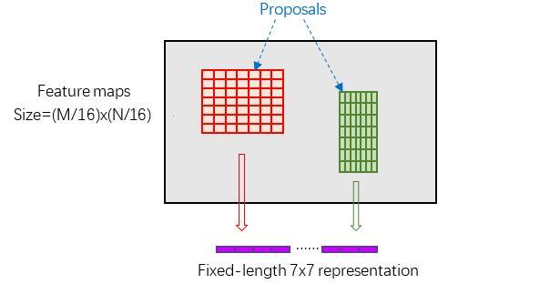图15 proposal示意图

4 Classification

Classification部分利用已经获得的proposal feature maps，通过full connect层与softmax计算每个proposal具体属于那个类别（如人，车，电视等），输出cls_prob概率向量；同时再次利用bounding box regression获得每个proposal的位置偏移量bbox_pred，用于回归更加精确的目标检测框。Classification部分网络结构如图16。

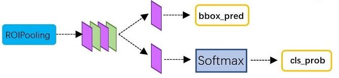图16 Classification部分网络结构图

从PoI Pooling获取到7x7=49大小的proposal feature maps后，送入后续网络，可以看到做了如下2件事：

通过全连接和softmax对proposals进行分类，这实际上已经是识别的范畴了
再次对proposals进行bounding box regression，获取更高精度的rect box

这里来看看全连接层InnerProduct layers，简单的示意图如图17，

图17 全连接层示意图

其计算公式如下：

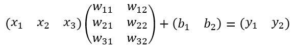
其中W和bias B都是预先训练好的，即大小是固定的，当然输入X和输出Y也就是固定大小。所以，这也就印证了之前Roi Pooling的必要性。到这里，我想其他内容已经很容易理解，不在赘述了。

5 Faster R-CNN训练

Faster R-CNN的训练，是在已经训练好的model（如VGG_CNN_M_1024，VGG，ZF）的基础上继续进行训练。实际中训练过程分为6个步骤：

在已经训练好的model上，训练RPN网络，对应stage1_rpn_train.pt
利用步骤1中训练好的RPN网络，收集proposals，对应rpn_test.pt
第一次训练Fast RCNN网络，对应stage1_fast_rcnn_train.pt
第二训练RPN网络，对应stage2_rpn_train.pt
再次利用步骤4中训练好的RPN网络，收集proposals，对应rpn_test.pt
第二次训练Fast RCNN网络，对应stage2_fast_rcnn_train.pt

可以看到训练过程类似于一种“迭代”的过程，不过只循环了2次。至于只循环了2次的原因是应为作者提到："A similar alternating training can be run for more iterations, but we have observed negligible improvements"，即循环更多次没有提升了。接下来本章以上述6个步骤讲解训练过程。

下面是一张训练过程流程图，应该更加清晰。

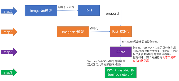图18 Faster RCNN训练步骤（引用自参考文章[1]）

5.1 训练RPN网络

在该步骤中，首先读取RBG提供的预训练好的model（本文使用VGG），开始迭代训练。来看看stage1_rpn_train.pt网络结构，如图19。

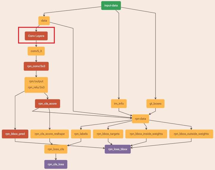图19 stage1_rpn_train.pt（考虑图片大小，Conv Layers中所有的层都画在一起了，如红圈所示，后续图都如此处理）

与检测网络类似的是，依然使用Conv Layers提取feature maps。整个网络使用的Loss如下：

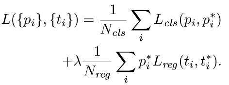
上述公式中， $i$ 表示anchors index， $p_{i}$ 表示foreground softmax probability， $p_{i}^{*}$ 代表对应的GT predict概率（即当第i个anchor与GT间 $IoU>0.7$ ，认为是该anchor是foreground， $p_{i}^{*}=1$ ；反之 $IoU<0.3$ 时，认为是该anchor是background， $p_{i}^{*}=0$ ；至于那些 $0.3<IoU<0.7$ 的anchor则不参与训练）； $t$ 代表predict bounding box， $t^{*}$ 代表对应foreground anchor对应的GT box。可以看到，整个Loss分为2部分：

cls loss，即rpn_cls_loss层计算的softmax loss，用于分类anchors为forground与background的网络训练
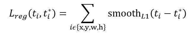
reg loss，即rpn_loss_bbox层计算的soomth L1 loss，用于bounding box regression网络训练。注意在该loss中乘了 $p_{i}^{*}$ ，相当于只关心foreground anchors的回归（其实在回归中也完全没必要去关心background）。

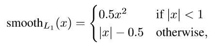
由于在实际过程中， $N_{cls}$ 和 $N_{reg}$ 差距过大，用参数λ平衡二者（如 $N_{cls}=256$ ， $N_{reg}=2400$ 时设置 $λ=10$ ），使总的网络Loss计算过程中能够均匀考虑2种Loss。这里比较重要是 $L_{reg}$ 使用的soomth L1 loss，计算公式如下：

了解数学原理后，反过来看图18：

在RPN训练阶段，rpn-data（python AnchorTargetLayer）层会按照和test阶段Proposal层完全一样的方式生成Anchors用于训练
对于rpn_loss_cls，输入的rpn_cls_scors_reshape和rpn_labels分别对应 $p$ 与 $p^{*}$ ， $N_{cls}$ 参数隐含在 $p$ 与 $p^{*}$ 的caffe blob的大小中
对于rpn_loss_bbox，输入的rpn_bbox_pred和rpn_bbox_targets分别对应 $t$ 于 $t^{*}$ ，rpn_bbox_inside_weigths对应 $p^{*}$ ，rpn_bbox_outside_weigths未用到（从soomth_L1_Loss layer代码中可以看到），而 $N_{reg}$ 同样隐含在caffe blob大小中

这样，公式与代码就完全对应了。特别需要注意的是，在训练和检测阶段生成和存储anchors的顺序完全一样，这样训练结果才能被用于检测！

5.2 通过训练好的RPN网络收集proposals

在该步骤中，利用之前的RPN网络，获取proposal rois，同时获取foreground softmax probability，如图20，然后将获取的信息保存在python pickle文件中。该网络本质上和检测中的RPN网络一样，没有什么区别。

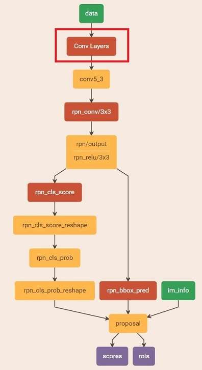图20 rpn_test.pt

5.3 训练Faster RCNN网络

读取之前保存的pickle文件，获取proposals与foreground probability。从data层输入网络。然后：

将提取的proposals作为rois传入网络，如图19蓝框
计算bbox_inside_weights+bbox_outside_weights，作用与RPN一样，传入soomth_L1_loss layer，如图20绿框

这样就可以训练最后的识别softmax与最终的bounding box regression了，如图21。

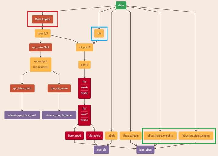图21 stage1_fast_rcnn_train.pt

之后的stage2训练都是大同小异，不再赘述了。Faster R-CNN还有一种end-to-end的训练方式，可以一次完成train，有兴趣请自己看作者GitHub吧。

Object Detection and Classification using R-CNNs

In this post, I’ll describe in detail how R-CNN (Regions with CNN features), a recently introduced deep learning based object detection and classification method works. R-CNN’s have proved highly effective in detecting and classifying objects in natural images, achieving mAP scores far higher than previous techniques. The R-CNN method is described in the following series of papers by Ross Girshick et al.

This post describes the final version of the R-CNN method described in the last paper. I considered at first to describe the evolution of the method from its first introduction to the final version, however that turned out to be a very ambitious undertaking. I settled on describing the final version in detail.

Fortunately, there are many implementations of the R-CNN algorithm available on the web in TensorFlow, PyTorch and other machine learning libraries. I used the following implementation:

https://github.com/ruotianluo/pytorch-faster-rcnn

Much of the terminology used in this post (for example the names of different layers) follows the terminology used in the code. Understanding the information presented in this post should make it much easier to follow the PyTorch implementation and make your own modifications.

Post Organization

Section 1 – Image Pre-Processing: In this section, we’ll describe the pre-processing steps that are applied to an input image. These steps include subtracting a mean pixel value and scaling the image. The pre-processing steps must be identical between training and inference
Section 2 – Network Organization: In this section, we’ll describe the three main components of the network – the “head” network, the region proposal network (RPN) and the classification network.
Section 3 – Implementation Details (Training): This is the longest section of the post and describes in detail the steps involved in training a R-CNN network
Section 4 – Implementation Details (Inference): In this section, we’ll describe the steps involved during inference – i.e., using the trained R-CNN network to identify promising regions and classify the objects in those regions.
Appendix: Here we’ll cover the details of some of the frequently used algorithms during the operation of a R-CNN such as non-maximum suppression and the details of the Resnet 50 architecture.

Image Pre-Processing

The following pre-processing steps are applied to an image before it is sent through the network. These steps must be identical for both training and inference. The mean vector ( $3 \times 1$ , one number corresponding to each color channel) is not the mean of the pixel values in the current image but a configuration value that is identical across all training and test images.

The default values for $targetSize$ and $maxSize$ parameters are 600 and 1000 respectively.

Network Organization

A R-CNN uses neural networks to solve two main problems:

Identify promising regions (Region of Interest – ROI) in an input image that are likely to contain foreground objects
Compute the object class probability distribution of each ROI – i.e., compute the probability that the ROI contains an object of a certain class. The user can then select the object class with the highest probability as the classification result.

R-CNNs consist of three main types of networks:

Head
Region Proposal Network (RPN)
Classification Network

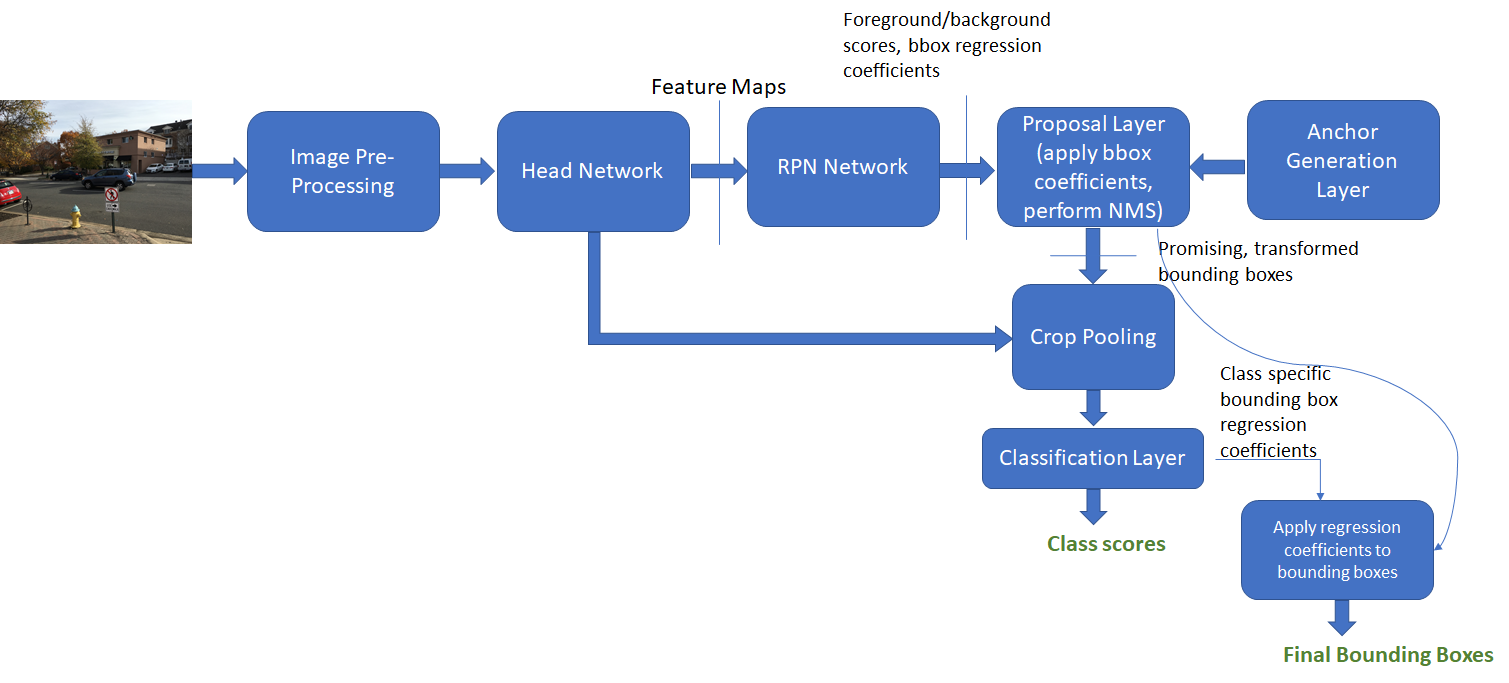
R-CNNs use the first few layers of a pre-trained network such as ResNet 50 to identify promising features from an input image. Using a network trained on one dataset on a different problem is possible because neural networks exhibit “transfer learning” (Yosinski et al. 2014)*. The first few layers of the network learn to detect general features such as edges and color blobs that are good discriminating features across many different problems. The features learnt by the later layers are higher level, more problem specific features. These layers can either be removed or the weights for these layers can be fine-tuned during back-propagation. The first few layers that are initialized from a pre-trained network constitute the “head” network. The convolutional feature maps produced by the head network are then passed through the Region Proposal Network (RPN) which uses a series of convolutional and fully connected layers to produce promising ROIs that are likely to contain a foreground object (problem 1 mentioned above). These promising ROIs are then used to crop out corresponding regions from the feature maps produced by the head network. This is called “Crop Pooling”. The regions produced by crop pooling are then passed through a classification network which learns to classify the object contained in each ROI.

As an aside, you may notice that weights for a ResNet are initialized in a curious way:

1 2	n = m.kernel_size[0] * m.kernel_size[1] * m.out_channels m.weight.data.normal_(0, math.sqrt(2. / n))

If you are interested in learning more about why this method works, read my post about initializing weights for convolutional and fully connected layers.

Network Architecture

The diagram below shows the individual components of the three network types described above. We show the dimensions of the input and output of each network layer which assists in understanding how data is transformed by each layer of the network. $w$ and $h$ represent the width and height of the input image (after pre-processing).

Implementation Details: Training

In this section, we’ll describe in detail the steps involved in training a R-CNN. Once you understand how training works, understanding inference is a lot easier as it simply uses a subset of the steps involved in training. The goal of training is to adjust the weights in the RPN and Classification network and fine-tune the weights of the head network (these weights are initialized from a pre-trained network such as ResNet). Recall that the job of the RPN network is to produce promising ROIs and the job of the classification network to assign object class scores to each ROI. Therefore, to train these networks, we need the corresponding ground truth i.e., the coordinates of the bounding boxes around the objects present in an image and the class of those objects. This ground truth comes from free to use image databases that come with an annotation file for each image. This annotation file contains the coordinates of the bounding box and the object class label for each object present in the image (the object classes are from a list of pre-defined object classes). These image databases have been used to support a variety of object classification and detection challenges. Two commonly used databases are:

PASCAL VOC: The VOC 2007 database contains 9963 training/validation/test images with 24,640 annotations for 20 object classes.
- Person: person
- Animal: bird, cat, cow, dog, horse, sheep
- Vehicle: aeroplane, bicycle, boat, bus, car, motorbike, train
- Indoor: bottle, chair, dining table, potted plant, sofa, tv/monitor

COCO (Common Objects in Context): The COCO dataset is much larger. It contains > 200K labelled images with 90 object categories.

I used the smaller PASCAL VOC 2007 dataset for my training. R-CNN is able to train both the region proposal network and the classification network in the same step.

Let’s take a moment to go over the concepts of “bounding box regression coefficients” and “bounding box overlap” that are used extensively in the remainder of this post.

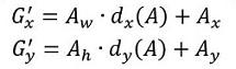
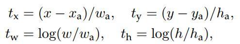
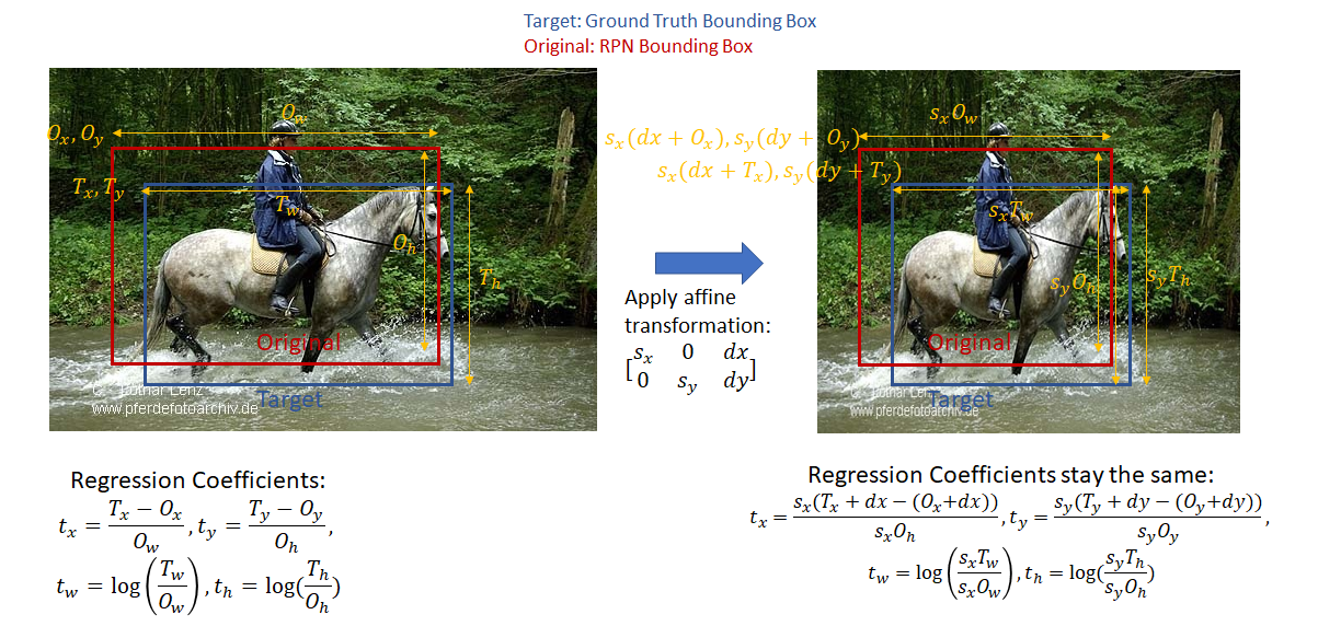
Bounding Box Regression Coefficients (also referred to as “regression coefficients” and “regression targets”): One of the goals of R-CNN is to produce good bounding boxes that closely fit object boundaries. R-CNN produces these bounding boxes by taking a given bounding box (defined by the coordinates of the top left corner, width and height) and tweaking its top left corner, width and height by applying a set of “regression coefficients”. These coefficients are computed as follows (Appendix C of (Anon. 2014)*. Let the x, y coordinates of the top left corner of the target and original bounding box be denoted by $T_x, T_y, O_x, O_y$ respectively and the width/height of the target and original bounding box by $T_w, T_h, O_w, O_h$ respectively. Then, the regression targets (coefficients of the function that transform the original bounding box to the target box) are given as:
- $t_x =\frac{(T_x - O_x)}{O_w}, t_y =\frac{(T_y - O_y)}{O_h}, t_w = log(\frac{T_w}{O_w}), t_h = log(\frac{T_h}{O_h})$ . This function is readily invertible, i.e., given the regression coefficients and coordinates of the top left corner and the width and height of the original bounding box, the top left corner and width and height of the target box can be easily calculated. Note the regression coefficients are invariant to an affine transformation with no shear. This is an important point as while calculating the classification loss, the target regression coefficients are calculated in the original aspect ratio while the classification network output regression coefficients are calculated after the ROI pooling step on square feature maps (1:1 aspect ratio). This will become clearer when we discuss classification loss below.
Intersection over Union (IoU) Overlap: We need some measure of how close a given bounding box is to another bounding box that is independent of the units used (pixels etc) to measure the dimensions of a bounding box. This measure should be intuitive (two coincident bounding boxes should have an overlap of 1 and two non-overlapping boxes should have an overlap of 0) and fast and easy to calculate. A commonly used overlap measure is the “Intersection over Union (IoU) overlap, calculated as shown below.

With these preliminaries out of the way, lets now dive into the implementation details for training a R-CNN. In the software implementation, R-CNN execution is broken down into several layers, as shown below. A layer encapsulates a sequence of logical steps that can involve running data through one of the neural networks and other steps such as comparing overlap between bounding boxes, performing non-maxima suppression etc.

Anchor Generation Layer: This layer generates a fixed number of “anchors” (bounding boxes) by first generating 9 anchors of different scales and aspect ratios and then replicating these anchors by translating them across uniformly spaced grid points spanning the input image.
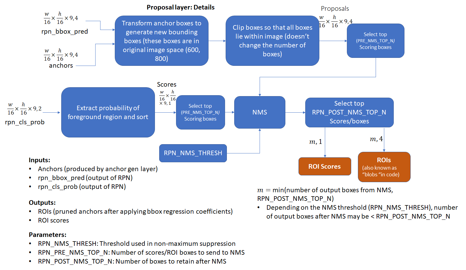
Proposal Layer: Transform the anchors according to the bounding box regression coefficients to generate transformed anchors. Then prune the number of anchors by applying non-maximum suppression (see Appendix) using the probability of an anchor being a foreground region
Anchor Target Layer: The goal of the anchor target layer is to produce a set of “good” anchors and the corresponding foreground/background labels and target regression coefficients to train the Region Proposal Network. The output of this layer is only used to train the RPN network and is not used by the classification layer. Given a set of anchors (produced by the anchor generation layer, the anchor target layer identifies promising foreground and background anchors. Promising foreground anchors are those whose overlap with some ground truth box is higher than a threshold. Background boxes are those whose overlap with any ground truth box is lower than a threshold. The anchor target layer also outputs a set of bounding box regressors i.e., a measure of how far each anchor target is from the closest bounding box. These regressors only make sense for the foreground boxes as there is no notion of “closest bounding box” for a background box.
RPN Loss: The RPN loss function is the metric that is minimized during optimization to train the RPN network. The loss function is a combination of:
- The proportion of bounding boxes produced by RPN that are correctly classified as foreground/background
- Some distance measure between the predicted and target regression coefficients.
Proposal Target Layer: The goal of the proposal target layer is to prune the list of anchors produced by the proposal layer and produce class specific bounding box regression targets that can be used to train the classification layer to produce good class labels and regression targets
ROI Pooling Layer: Implements a spatial transformation network that samples the input feature map given the bounding box coordinates of the region proposals produced by the proposal target layer. These coordinates will generally not lie on integer boundaries, thus interpolation based sampling is required.
Classification Layer: The classification layer takes the output feature maps produced by the ROI Pooling Layer and passes them through a series of convolutional layers. The output is fed through two fully connected layers. The first layer produces the class probability distribution for each region proposal and the second layer produces a set of class specific bounding box regressors.
Classification Loss: Similar to RPN loss, classification loss is the metric that is minimized during optimization to train the classification network. During back propagation, the error gradients flow to the RPN network as well, so training the classification layer modifies the weights of the RPN network as well. We’ll have more to say about this point later. The classification loss is a combination of:
- The proportion of bounding boxes produced by RPN that are correctly classified (as the correct object class)
- Some distance measure between the predicted and target regression coefficients.

We’ll now go through each of these layers in detail.

Anchor Generation Layer

The anchor generation layer produces a set of bounding boxes (called “anchor boxes”) of varying sizes and aspect ratios spread all over the input image. These bounding boxes are the same for all images i.e., they are agnostic of the content of an image. Some of these bounding boxes will enclose foreground objects while most won’t. The goal of the RPN network is to learn to identify which of these boxes are good boxes – i.e., likely to contain a foreground object and to produce target regression coefficients, which when applied to an anchor box turns the anchor box into a better bounding box (fits the enclosed foreground object more closely).

The diagram below demonstrates how these anchor boxes are generated.

Region Proposal Layer

Object detection methods need as input a “region proposal system” that produces a set of sparse (for example selective search (Anon.)*) or a dense (for example features used in deformable part models (Anon.)*) set of features. The first version of the R-CNN system used the selective search method for generating region proposal. In the current version (known as “Faster R-CNN”), a “sliding window” based technique (described in the previous section) is used to generate a set of dense candidate regions and then a neural network driven region proposal network is used to rank region proposals according to the probability of a region containing a foreground object. The region proposal layer has two goals:

From a list of anchors, identify background and foreground anchors
Modify the position, width and height of the anchors by applying a set of “regression coefficients” to improve the quality of the anchors (for example, make them fit the boundaries of objects better)

The region proposal layer consists of a Region Proposal Network and three layers – Proposal Layer, Anchor Target Layer and Proposal Target Layer. These three layers are described in detail in the following sections.

Region Proposal Network

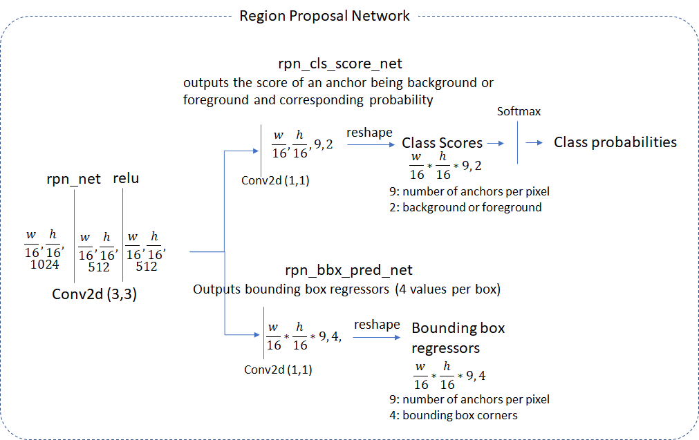
The region proposal layer runs feature maps produced by the head network through a convolutional layer (called rpn_net in code) followed by RELU. The output of rpn_net is run through two (1,1) kernel convolutional layers to produce background/foreground class scores and probabilities and corresponding bounding box regression coefficients. The stride length of the head network matches the stride used while generating the anchors, so the number of anchor boxes are in 1-1 correspondence with the information produced by the region proposal network (number of anchor boxes = number of class scores = number of bounding box regression coefficients = $\frac{w}{16}\times\frac{h}{16}\times9$ )

Proposal Layer

The proposal layer takes the anchor boxes produced by the anchor generation layer and prunes the number of boxes by applying non-maximum suppression based on the foreground scores (see appendix for details). It also generates transformed bounding boxes by applying the regression coefficients generated by the RPN to the corresponding anchor boxes.

Anchor Target Layer

The goal of the anchor target layer is to select promising anchors that can be used to train the RPN network to:

distinguish between foreground and background regions and
generate good bounding box regression coefficients for the foreground boxes.

It is useful to first look at how the RPN Loss is calculated. This will reveal the information needed to calculate the RPN loss which makes it easy to follow the operation of the Anchor Target Layer.

Calculating RPN Loss

Remember the goal of the RPN layer is to generate good bounding boxes. To do so from a set of anchor boxes, the RPN layer must learn to classify an anchor box as background or foreground and calculate the regression coefficients to modify the position, width and height of a foreground anchor box to make it a “better” foreground box (fit a foreground object more closely). RPN Loss is formulated in such a way to encourage the network to learn this behaviour.

RPN loss is a sum of the classification loss and bounding box regression loss. The classification loss uses cross entropy loss to penalize incorrectly classified boxes and the regression loss uses a function of the distance between the true regression coefficients (calculated using the closest matching ground truth box for a foreground anchor box) and the regression coefficients predicted by the network (see rpn_bbx_pred_net in the RPN network architecture diagram).

$RPN Loss = \text{Classification Loss} + \text{Bounding Box Regression Loss}$

Classification Loss:

cross_entropy(predicted _class, actual_class)

Bounding Box Regression Loss:

$L_{loc} = \sum_{u \in {\text{all foreground anchors}}}l_u$

Sum over the regression losses for all foreground anchors. Doing this for background anchors doesn’t make sense as there is no associated ground truth box for a background anchor

$l_u = \sum_{i \in {x,y,w,h}}smooth_{L1}(u_i(predicted)-u_i(target))$

This shows how the regression loss for a given foreground anchor is calculated. We take the difference between the predicted (by the RPN) and target (calculated using the closest ground truth box to the anchor box) regression coefficients. There are four components – corresponding to the coordinates of the top left corner and the width/height of the bounding box. The smooth L1 function is defined as follows:

$smooth_{L1}(x) = \begin{cases} \frac{\sigma^2x^2}{2} & \lVert x \rVert < \frac{1}{\sigma^2} \\ \lVert x \rVert - \frac{0.5}{\sigma^2} & otherwise\end{cases}$

Here $\sigma$ is chosen arbitrarily (set to 3 in my code). Note that in the python implementation, a mask array for the foreground anchors (called “bbox_inside_weights”) is used to calculate the loss as a vector operation and avoid for-if loops.

Thus, to calculate the loss we need to calculate the following quantities:

Class labels (background or foreground) and scores for the anchor boxes
Target regression coefficients for the foreground anchor boxes

We’ll now follow the implementation of the anchor target layer to see how these quantities are calculated. We first select the anchor boxes that lie within the image extent. Then, good foreground boxes are selected by first computing the IoU (Intersection over Union) overlap of all anchor boxes (within the image) with all ground truth boxes. Using this overlap information, two types of boxes are marked as foreground:

type A: For each ground truth box, all foreground boxes that have the max IoU overlap with the ground truth box
type B: Anchor boxes whose maximum overlap with some ground truth box exceeds a threshold

these boxes are shown in the image below:

Note that only anchor boxes whose overlap with some ground truth box exceeds a threshold are selected as foreground boxes. This is done to avoid presenting the RPN with the “hopeless learning task” of learning the regression coefficients of boxes that are too far from the best match ground truth box. Similarly, boxes whose overlap are less than a negative threshold are labeled background boxes. Not all boxes that are not foreground boxes are labeled background. Boxes that are neither foreground or background are labeled “don’t care”. These boxes are not included in the calculation of RPN loss.

There are two additional thresholds related to the total number of background and foreground boxes we want to achieve and the fraction of this number that should be foreground. If the number of foreground boxes that pass the test exceeds the threshold, we randomly mark the excess foreground boxes to “don’t care”. Similar logic is applied to the background boxes.

Next, we compute bounding box regression coefficients between the foreground boxes and the corresponding ground truth box with maximum overlap. This is easy and one just needs to follow the formula to calculate the regression coefficients.

This concludes our discussion of the anchor target layer. To recap, let’s list the parameters and input/output for this layer:

Parameters:

TRAIN.RPN_POSITIVE_OVERLAP: Threshold used to select if an anchor box is a good foreground box (Default: 0.7)
TRAIN.RPN_NEGATIVE_OVERLAP: If the max overlap of a anchor from a ground truth box is lower than this thershold, it is marked as background. Boxes whose overlap is > than RPN_NEGATIVE_OVERLAP but < RPN_POSITIVE_OVERLAP are marked “don’t care”.(Default: 0.3)
TRAIN.RPN_BATCHSIZE: Total number of background and foreground anchors (default: 256)
TRAIN.RPN_FG_FRACTION: fraction of the batch size that is foreground anchors (default: 0.5). If the number of foreground anchors found is larger than TRAIN.RPN_BATCHSIZE $\times$ TRAIN.RPN_FG_FRACTION, the excess (indices are selected randomly) is marked “don’t care”.

Input:

RPN Network Outputs (predicted foreground/background class labels, regression coefficients)
Anchor boxes (generated by the anchor generation layer)
Ground truth boxes

Output

Good foreground/background boxes and associated class labels
Target regression coefficients

The other layers, proposal target layer, ROI Pooling layer and classification layer are meant to generate the information needed to calculate classification loss. Just as we did for the anchor target layer, let’s first look at how classification loss is calculated and what information is needed to calculate it

Calculating Classification Layer Loss

Similar to the RPN Loss, classification layer loss has two components – classification loss and bounding box regression loss

$\text{Classification Layer Loss} = \text{Classification Loss} + \text{Bounding Box Regression Loss}$

The key difference between the RPN layer and the classification layer is that while the RPN layer dealt with just two classes – foreground and background, the classification layer deals with all the object classes (plus background) that our network is being trained to classify.

The classification loss is the cross entropy loss with the true object class and predicted class score as the parameters. It is calculated as shown below.

The bounding box regression loss is also calculated similar to the RPN except now the regression coefficients are class specific. The network calculates regression coefficients for each object class. The target regression coefficients are obviously only available for the correct class which is the object class of the ground truth bounding box that has the maximum overlap with a given anchor box. While calculating the loss, a mask array which marks the correct object class for each anchor box is used. The regression coefficients for the incorrect object classes are ignored. This mask array allows the computation of loss to be a matrix multiplication as opposed to requiring a for-each loop.

Thus the following quantities are needed to calculate classification layer loss:

Predicted class labels and bounding box regression coefficients (these are outputs of the classification network)
class labels for each anchor box
Target bounding box regression coefficients

Let’s now look at how these quantities are calculated in the proposal target and classification layers.

Proposal Target Layer

The goal of the proposal target layer is to select promising ROIs from the list of ROIs output by the proposal layer. These promising ROIs will be used to perform crop pooling from the feature maps produced by the head layer and passed to the rest of the network (head_to_tail) that calculates predicted class scores and box regression coefficients.

Similar to the anchor target layer, it is important to select good proposals (those that have significant overlap with gt boxes) to pass on to the classification layer. Otherwise, we’ll be asking the classification layer to learn a “hopeless learning task”.

The proposal target layer starts with the ROIs computed by the proposal layer. Using the max overlap of each ROI with all ground truth boxes, it categorizes the ROIs into background and foreground ROIs. Foreground ROIs are those for which max overlap exceeds a threshold (TRAIN.FG_THRESH, default: 0.5). Background ROIs are those whose max overlap falls between TRAIN.BG_THRESH_LO and TRAIN.BG_THRESH_HI (default 0.1, 0.5 respectively). This is an example of “hard negative mining” used to present difficult background examples to the classifier.

There is some additional logic that tries to make sure that the total number of foreground and background region is constant. In case too few background regions are found, it tries to fill in the batch by randomly repeating some background indices to make up for the shortfall.

Next, bounding box target regression targets are computed between each ROI and the closest matching ground truth box (this includes the background ROIs also, as an overlapping ground truth box exists for these ROIs also). These regression targets are expanded for all classes as shown in the figure below.

the bbox_inside_weights array acts as a mask. It is 1 only for the correct class for each foreground ROI. It is zero for the background ROIs as well. Thus, while computing the bounding box regression component of the classification layer loss, only the regression coefficients for the foreground regions are taken into account. This is not the case for the classification loss – the background ROIs are included as well as they belong to the “background” class.

Input:

ROIs produced by the proposal layer
ground truth information

Output:

Selected foreground and background ROIs that meet overlap criteria.
Class specific target regression coefficients for the ROIs

Parameters:

TRAIN.FG_THRESH: (default: 0.5) Used to select foreground ROIs. ROIs whose max overlap with a ground truth box exceeds FG_THRESH are marked foreground
TRAIN.BG_THRESH_HI: (default 0.5)
TRAIN.BG_THRESH_LO: (default 0.1) These two thresholds are used to select background ROIs. ROIs whose max overlap falls between BG_THRESH_HI and BG_THRESH_LO are marked background
TRAIN.BATCH_SIZE: (default 128) Maximum number of foreground and background boxes selected.
TRAIN.FG_FRACTION: (default 0.25). Number of foreground boxes can’t exceed BATCH_SIZE*FG_FRACTION

Crop Pooling

Proposal target layer produces promising ROIs for us to classify along with the associated class labels and regression coefficients that are used during training. The next step is to extract the regions corresponding to these ROIs from the convolutional feature maps produced by the head network. The extracted feature maps are then run through the rest of the network (“tail” in the network diagram shown above) to produce object class probability distribution and regression coefficients for each ROI. The job of the Crop Pooling layer is to perform region extraction from the convolutional feature maps.

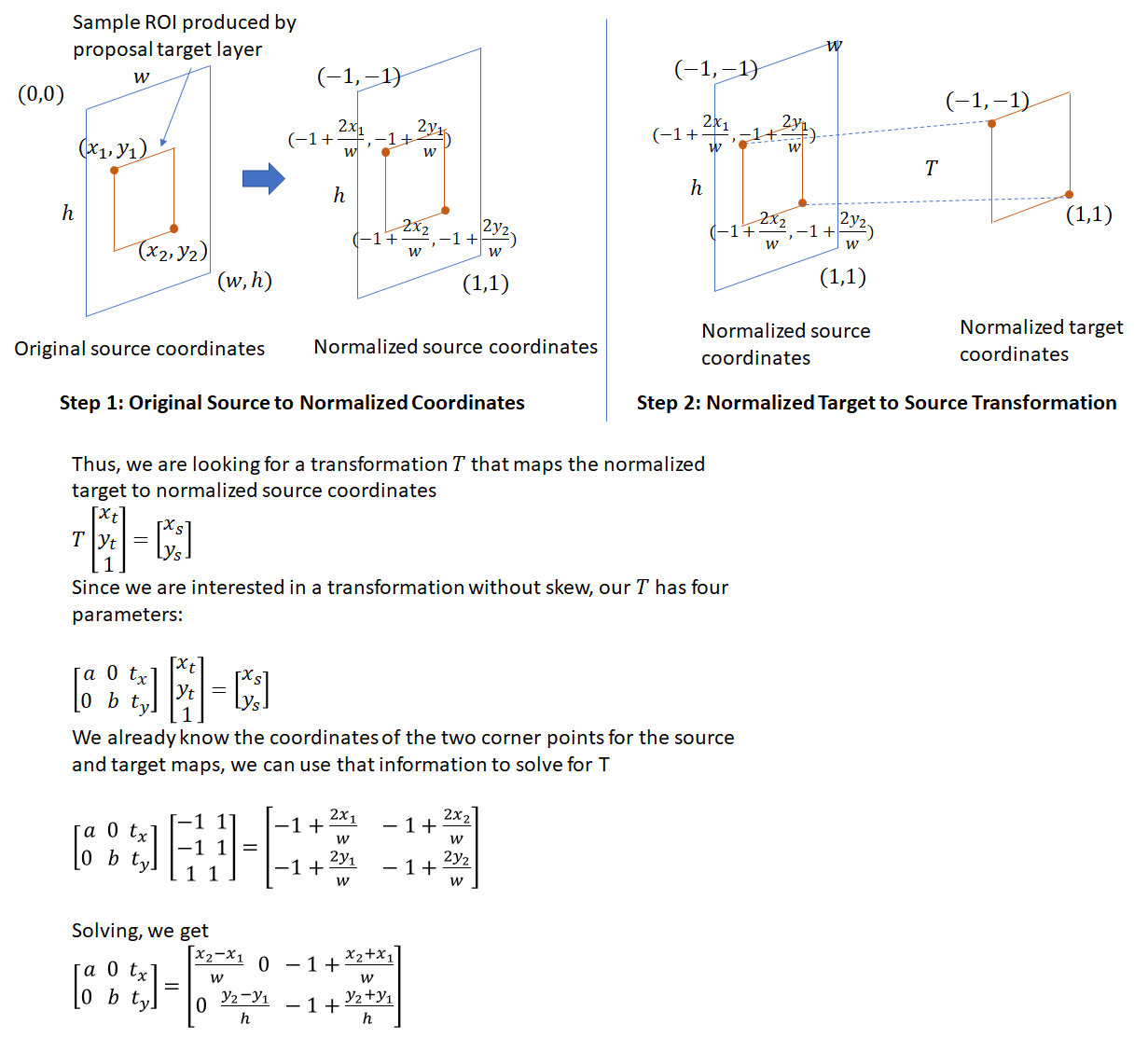
The key ideas behind crop pooling are described in the paper on “Spatial Transformation Networks” (Anon. 2016)*. The goal is to apply a warping function (described by a $2\times 3$ affine transformation matrix) to an input feature map to output a warped feature map. This is shown in the figure below

There are two steps involved in crop pooling:

For a set of target coordinates, apply the given affine transformation to produce a grid of source coordinates.
$\begin{bmatrix} x_i^s \\ y_i^s \end{bmatrix} = \begin{bmatrix} \theta_{11} & \theta_{12} & \theta_{13} \\ \theta_{21} & \theta_{22} & \theta_{23} \end{bmatrix}\begin{bmatrix} x_i^t \\ y_i^t \\ 1\end{bmatrix}$ . Here $x_i^s, y_i^s, x_i^t, y_i^t$ are height/width normalized coordinates (similar to the texture coordinates used in graphics), so $-1 \leq x_i^s, y_i^s, x_i^t, y_i^t \leq 1$ .
In the second step, the input (source) map is sampled at the source coordinates to produce the output (destination) map. In this step, each $(x_i^s, y_i^s)$ coordinate defines the spatial location in the input where a sampling kernel (for example bi-linear sampling kernel) is applied to get the value at a particular pixel in the output feature map.

The sampling methodology described in the spatial transformation gives a differentiable sampling mechanism allowing for loss gradients to flow back to the input feature map and the sampling grid coordinates.

Fortunately, crop pooling is implementated in PyTorch and the API consists of two functions that mirror these two steps. torch.nn.functional.affine_gridtakes an affine transformation matrix and produces a set of sampling coordinates and torch.nn.functional.grid_sample samples the grid at those coordinates. Back-propagating gradients during the backward step is handled automatically by pyTorch.

To use crop pooling, we need to do the following:

Divide the ROI coordinates by the stride length of the “head” network. The coordinates of the ROIs produced by the proposal target layer are in the original image space (! 800 $\times$ 600). To bring these coordinates into the space of the output feature maps produced by “head”, we must divide them by the stride length (16 in the current implementation).
To use the API shown above, we need the affine transformation matrix. This affine transformation matrix is computed as shown below
We also need the number of points in the $x$ and $y$ dimensions on the target feature map. This is provided by the configuration parameter cfg.POOLING_SIZE (default 7). Thus, during crop pooling, non-square ROIs are used to crop out regions from the convolution feature map which are warped to square windows of constant size. This warping must be done as the output of crop pooling is passed to further convolutional and fully connected layers which need input of a fixed dimension.

Classification Layer

The crop pooling layer takes the ROI boxes output by the proposal target layer and the convolutional feature maps output by the “head” network and outputs square feature maps. The feature maps are then passed through layer 4 of ResNet following by average pooling along the spatial dimensions. The result (called “fc7” in code) is a one-dimensional feature vector for each ROI. This process is shown below.

The feature vector is then passed through two fully connected layers – bbox_pred_net and cls_score_net. The cls_score_net layer produces the class scores for each bounding box (which can be converted into probabilities by applying softmax). The bbox_pred_net layer produces the class specific bounding box regression coefficients which are combined with the original bounding box coordinates produced by the proposal target layer to produce the final bounding boxes. These steps are shown below.

It’s good to recall the difference between the two sets of bounding box regression coefficients – one set produced by the RPN network and the second set produced by the classification network. The first set is used to train the RPN layer to produce good foreground bounding boxes (that fit more tightly around object boundaries). The target regression coefficients i.e., the coefficients needed to align a ROI box with its closest matching ground truth bounding box are generated by the anchor target layer. It is difficult to identify precisely how this learning takes place, but I’d imagine the RPN convolutional and fully connected layers learn how to interpret the various image features generated by the neural network into deciphering good object bounding boxes. When we consider Inference in the next section, we’ll see how these regression coefficients are used.

The second set of bounding box coefficients is generated by the classification layer. These coefficients are class specific, i.e., one set of coefficients are generated per object class for each ROI box. The target regression coefficients for these are generated by the proposal target layer. Note that the classification network operates on square feature maps that are a result of the affine transformation (described above) applied to the head network output. However since the regression coefficients are invariant to an affine transformation with no shear, the target regression coefficients computed by the proposal target layer can be compared with those produced by the classification network and act as a valid learning signal. This point seems obvious in hindsight, but took me some time to understand.

It is interesting to note that while training the classification layer, the error gradients propagate to the RPN network as well. This is because the ROI box coordinates used during crop pooling are themselves network outputs as they are a result of applying the regression coefficients generated by the RPN network to the anchor boxes. During back-propagation, the error gradients will propagate back through the crop-pooling layer to the RPN layer. Calculating and applying these gradients would be quite tricky to implement, however thankfully the crop pooling API is provided by PyTorch as a built-in module and the details of calculating and applying the gradients are handled internally. This point is discussed in Section 3.2 (iii) of the Faster RCNN paper (Ren et al. 2015)*.

Implementation Details: Inference

The steps carried out during inference are shown below

Anchor target and proposal target layers are not used. The RPN network is supposed to have learnt how to classify the anchor boxes into background and foreground boxes and generate good bounding box coefficients. The proposal layer simply applies the bounding box coefficients to the top ranking anchor boxes and performs NMS to eliminate boxes with a large amount of overlap. The output of these steps are shown below for additional clarity. The resulting boxes are sent to the classification layer where class scores and class specific bounding box regression coefficients are generated.

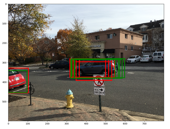The red boxes show the top 6 anchors ranked by score. Green boxes show the anchor boxes after applying the regression parameters computed by the RPN network. The green boxes appear to fit the underlying object more tightly. Note that after applying the regression parameters, a rectangle remains a rectangle, i.e., there is no shear. Also note the significant overlap between rectangles. This redundancy is addressed by applying non-maxima suppression

Red boxes show the top 5 bounding boxes before NMS, green boxes show the top 5 boxes after NMS. By suppressing overlapping boxes, other boxes (lower in the scores list) get a chance to move up

From the final classification scores array (dim: n, 21), we select the column corresponding to a certain foreground object, say car. Then, we select the row corresponding to the max score in this array. This row corresponds to the proposal that is most likely to be a car. Let the index of this row be car_score_max_idx Now, let the array of final bounding box coordinates (after applying the regression coefficients) be bboxes (dim: n,21*4). From this array, we select the row corresponding to car_score_max_idx. We expect that the bounding box corresponding to the car column should fit the car in the test image better than the other bounding boxes (which correspond to the wrong object classes). This is indeed the case. The red box corresponds to the original proposal box, the blue box is the calculated bounding box for the car class and the white boxes correspond to the other (incorrect) foreground classes. It can be seen that the blue box fits the actual car better than the other boxes.

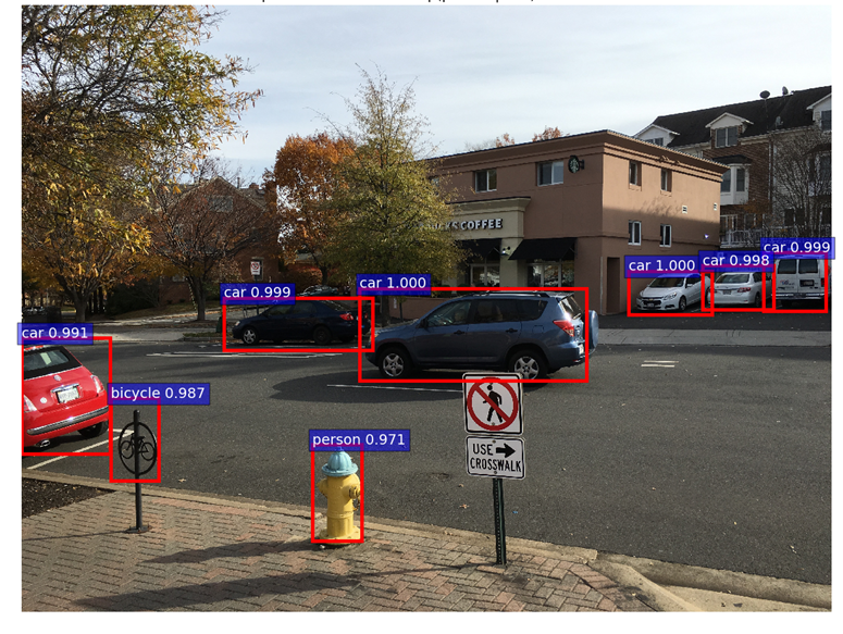
For showing the final classification results, we apply another round of NMS and apply an object detection threshold to the class scores. We then draw all transformed bounding boxes corresponding to the ROIs that meet the detection threshold. The result is shown below.

Appendix

ResNet 50 Network Architecture

Non-Maximum Suppression (NMS)

Non-maximum suppression is a technique used to reduce the number of candidate boxes by eliminating boxes that overlap by an amount larger than a threhold. The boxes are first sorted by some criteria (usually the y coordinate of the bottom right corner). We then go through the list of boxes and suppress those boxes whose IoU overlap with the box under consideration exceeds a threshold. Sorting the boxes by the y coordinate results in the lowest box among a set of overlapping boxes being retained. This may not always be the desired outcome. NMS used in R-CNN sorts the boxes by the foreground score. This results in the box with the highest score among a set of overlapping boxes being retained. The figures below show the difference between the two approaches. The numbers in black are the foreground scores for each box. The image on the right shows the result of applying NMS to the image on left. The first figure uses standard NMS (boxes are ranked by y coordinate of bottom right corner). This results in the box with a lower score being retained. The second figure uses modified NMS (boxes are ranked by foreground scores). This results in the box with the highest foreground score being retained, which is more desirable. In both cases, the overlap between the boxes is assumed to be higher than the NMS overlap threhold.

Bibliography

Anon. 2014. . October 23. https://arxiv.org/pdf/1311.2524.pdf.

Anon. 2016. . February 5. https://arxiv.org/pdf/1506.02025.pdf.

Anon. . http://link.springer.com/article/10.1007/s11263-013-0620-5.

Anon. Object Detection with Discriminatively Trained Part-Based Models - IEEE Journals & Magazine. https://doi.org/10.1109/TPAMI.2009.167.

Girshick, Ross. 2015. Fast R-CNN. arXiv.org. April 30. https://arxiv.org/abs/1504.08083.

Girshick, Ross, Jeff Donahue, Trevor Darrell, and Jitendra Malik. 2013. Rich feature hierarchies for accurate object detection and semantic segmentation. arXiv.org. November 11. https://arxiv.org/abs/1311.2524.

Ren, Shaoqing, Kaiming He, Ross Girshick, and Jian Sun. 2015. Faster R-CNN: Towards Real-Time Object Detection with Region Proposal Networks. arXiv.org. June 4. https://arxiv.org/abs/1506.01497.

Yosinski, Jason, Jeff Clune, Yoshua Bengio, and Hod Lipson. 2014. How transferable are features in deep neural networks? arXiv.org. November 6. https://arxiv.org/abs/1411.1792.

posted on 2018-10-02 23:18 Satchmo丶阅读(1042) 评论(0) 编辑收藏举报