关于torchvision.models中VGG的笔记

VGG 主要有两种结构，分别是 VGG16 和 VGG19，两者并没有本质上的区别，只是网络深度不一样。

对于给定的感受野，采用堆积的小卷积核是优于采用大的卷积核的，因为多层非线性层可以增加网络深度来保证学习更复杂的模式，而且代价还比较小（参数更少）。

比如，三个步长为 $1$ 的 $3 \times 3$ 卷积核的叠加，即对应 $7 \times 7$ 的感受野（即三个 $3 \times 3$ 连续卷积相当于一个 $7 \times 7$ 卷积），如果我们假设卷积输入输出的 channel 数均为 $C$，那么三个 $3 \times 3$ 连续卷积的参数总量为 $3 \times (9 C^2)$（一个卷积核的大小 $3 \times 3 \times C$，一层有 $C$ 个卷积核，总共有三层），而如果直接使用 $7 \times 7$ 卷积核，其参数总量为 $49 C^2$。很明显 $27C^2 < 49C^2$，即减少了参数。

VGG的网络结构非常简单，全部都是 $(3,3)$ 的卷积核，步长为 $1$，四周补 $1$ 圈 $0$（使得输入输出的 $(H,W)$ 不变）：

 

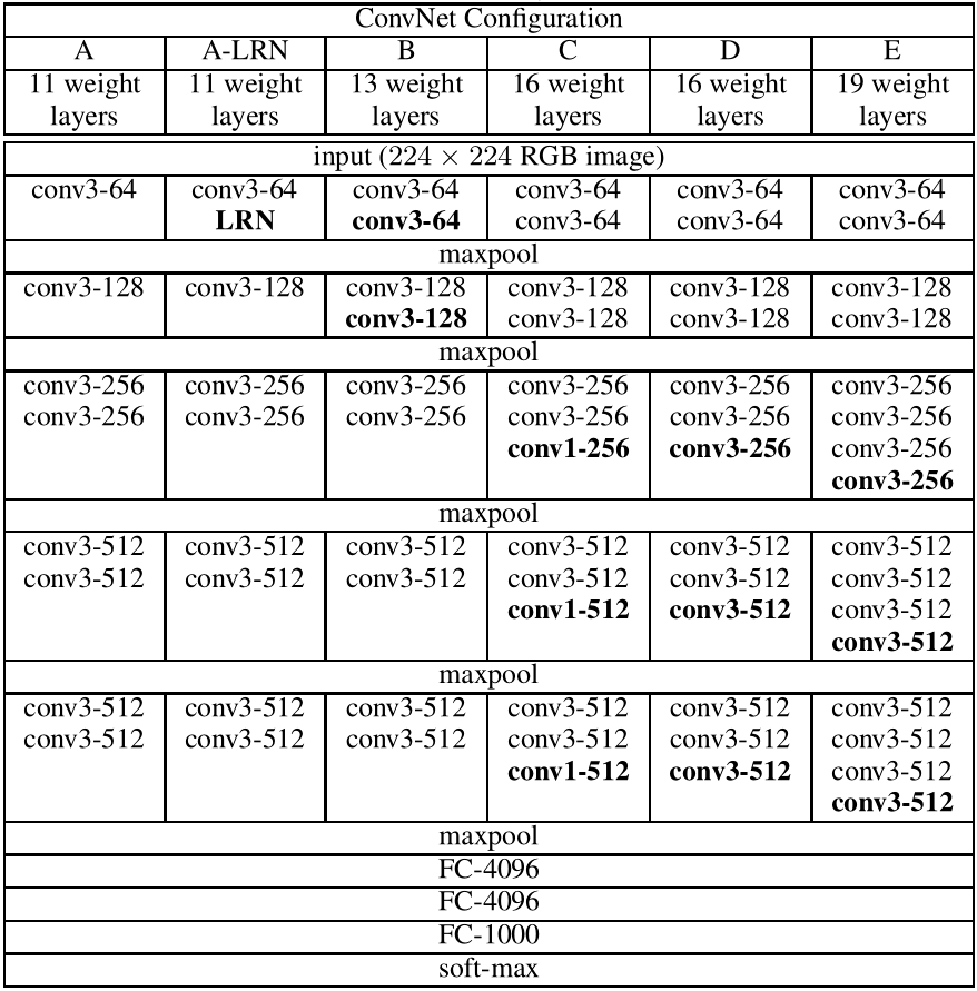
我们可以参考 torchvision.models 中的源码：

class VGG(nn.Module):

    def __init__(self, features, num_classes=1000, init_weights=True):
        super(VGG, self).__init__()
        self.features = features
        self.avgpool = nn.AdaptiveAvgPool2d((7, 7))
        self.classifier = nn.Sequential(
            nn.Linear(512 * 7 * 7, 4096),
            nn.ReLU(True),
            nn.Dropout(),
            nn.Linear(4096, 4096),
            nn.ReLU(True),
            nn.Dropout(),
            nn.Linear(4096, num_classes),
        )
        if init_weights:
            self._initialize_weights()

    def forward(self, x):
        x = self.features(x)
        x = self.avgpool(x)
        x = torch.flatten(x, 1)
        x = self.classifier(x)
        return x

    def _initialize_weights(self):
        for m in self.modules():
            if isinstance(m, nn.Conv2d):
                nn.init.kaiming_normal_(m.weight, mode='fan_out', nonlinearity='relu')
                if m.bias is not None:
                    nn.init.constant_(m.bias, 0)
            elif isinstance(m, nn.BatchNorm2d):
                nn.init.constant_(m.weight, 1)
                nn.init.constant_(m.bias, 0)
            elif isinstance(m, nn.Linear):
                nn.init.normal_(m.weight, 0, 0.01)
                nn.init.constant_(m.bias, 0)


def make_layers(cfg, batch_norm=False):
    layers = []
    in_channels = 3
    for v in cfg:
        if v == 'M':
            layers += [nn.MaxPool2d(kernel_size=2, stride=2)]
        else:
            conv2d = nn.Conv2d(in_channels, v, kernel_size=3, padding=1)
            if batch_norm:
                layers += [conv2d, nn.BatchNorm2d(v), nn.ReLU(inplace=True)]
            else:
                layers += [conv2d, nn.ReLU(inplace=True)]
            in_channels = v
    return nn.Sequential(*layers)


cfgs = {
    'A': [64, 'M', 128, 'M', 256, 256, 'M', 512, 512, 'M', 512, 512, 'M'],
    'B': [64, 64, 'M', 128, 128, 'M', 256, 256, 'M', 512, 512, 'M', 512, 512, 'M'],
    'D': [64, 64, 'M', 128, 128, 'M', 256, 256, 256, 'M', 512, 512, 512, 'M', 512, 512, 512, 'M'],
    'E': [64, 64, 'M', 128, 128, 'M', 256, 256, 256, 256, 'M', 512, 512, 512, 512, 'M', 512, 512, 512, 512, 'M'],
}


def _vgg(arch, cfg, batch_norm, pretrained, progress, **kwargs):
    if pretrained:
        kwargs['init_weights'] = False
    model = VGG(make_layers(cfgs[cfg], batch_norm=batch_norm), **kwargs)
    if pretrained:
        state_dict = load_state_dict_from_url(model_urls[arch],
                                              progress=progress)
        model.load_state_dict(state_dict)
    return model

cfgs 中的 "A,B,D,E" 就分别对应上表中的 A,B,D,E 四种网络结构。

'M' 代表最大池化层， nn.MaxPool2d(kernel_size=2, stride=2) 

从代码中可以看出，经过 self.features 的一大堆卷积层之后，先是经过一个 nn.AdaptiveAvgPool2d((7, 7)) 的自适应平均池化层（自动选择参数使得输出的 tensor 满足 $(H = 7,W = 7)$），再通过一个 torch.flatten(x, 1) 推平成一个 $(batch\_size, n)$ 的 tensor，再连接后面的全连接层。

 

torchvision.models.vgg19_bn(pretrained=False, progress=True, **kwargs)

pretrained: 如果设置为 True，则返回在 ImageNet 预训练过的模型。