

Pytorch-GAN
任务:使用8个高斯混合模型生成一系列数据,通过GAN学习它的分布,比较学习的分布和真实的分布是否一样。
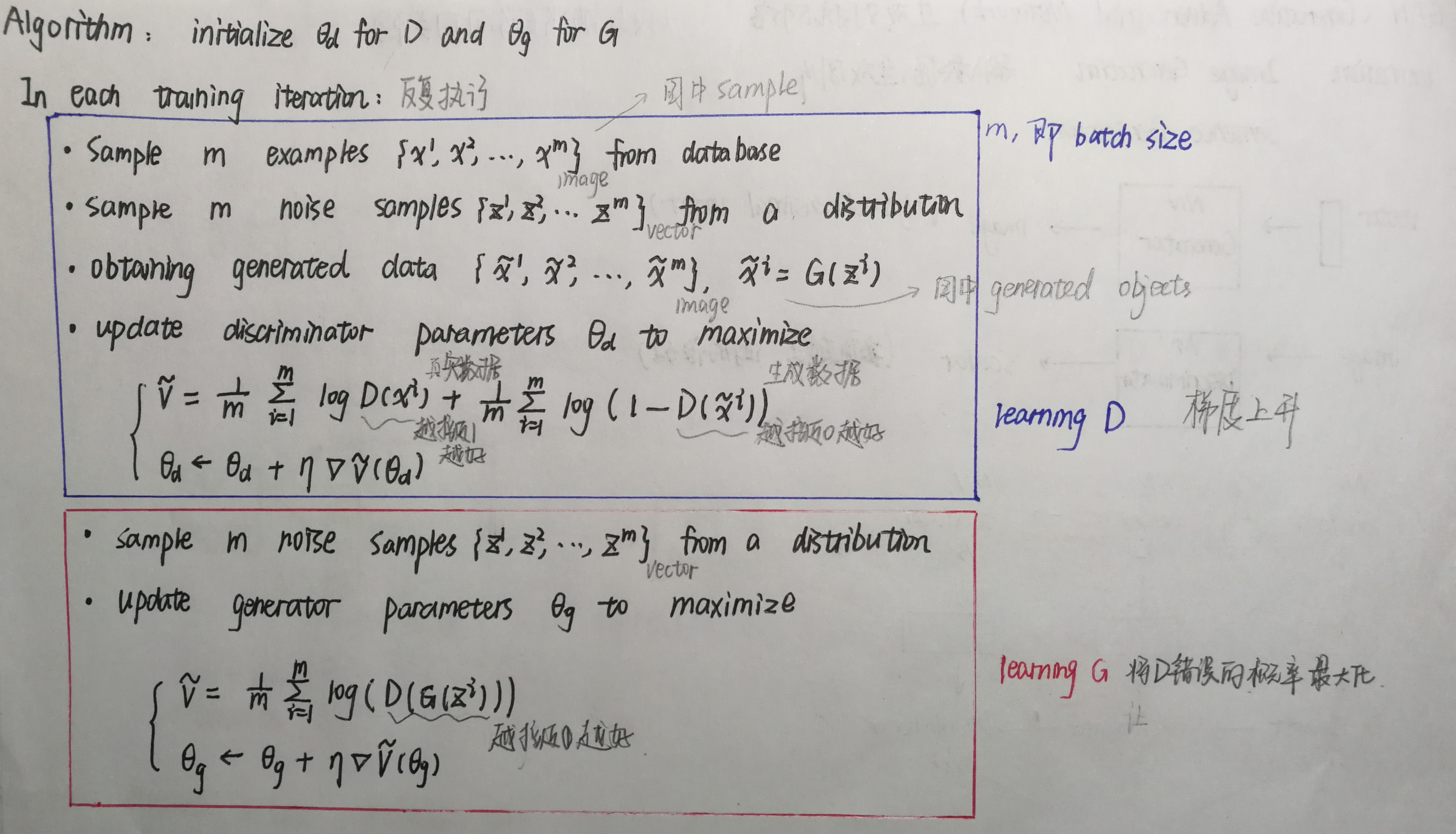
GAN文字版算法:

GAN公式版算法:
在命令行执行如下语句(详细Visdom的使用见https://www.cnblogs.com/cxq1126/p/13285150.html)
python -m visidom.server
提前导包:
 1 import  torch
 2 from    torch import nn, optim, autograd
 3 import  numpy as np
 4 import  visdom
 5 from    torch.nn import functional as F
 6 from    matplotlib import pyplot as plt
 7 import  random
 8
 9 h_dim = 400
10 batchsz = 512
11 viz = visdom.Visdom()
1.实现Generator
输入点坐标,输出点坐标。
 1 class Generator(nn.Module):
 2
 3     def __init__(self):
 4         super(Generator, self).__init__()
 5
 6         self.net = nn.Sequential(
 7             nn.Linear(2, h_dim),
 8             nn.ReLU(True),
 9             nn.Linear(h_dim, h_dim),
10             nn.ReLU(True),
11             nn.Linear(h_dim, h_dim),
12             nn.ReLU(True),
13             nn.Linear(h_dim, 2),
14         )
15
16     def forward(self, z):
17         output = self.net(z)
18         return output
2.实现Discriminator
输入点坐标,输出数值(用来评判输入的坐标是否在真实数据附近)。
 1 class Discriminator(nn.Module):
 2
 3     def __init__(self):
 4         super(Discriminator, self).__init__()
 5
 6         self.net = nn.Sequential(
 7             nn.Linear(2, h_dim),
 8             nn.ReLU(True),
 9             nn.Linear(h_dim, h_dim),
10             nn.ReLU(True),
11             nn.Linear(h_dim, h_dim),
12             nn.ReLU(True),
13             nn.Linear(h_dim, 1),
14             nn.Sigmoid()
15         )
16
17     def forward(self, x):
18         output = self.net(x)
19         return output.view(-1)
3.权重初始化
1 def weights_init(m):
2     if isinstance(m, nn.Linear):
3         # m.weight.data.normal_(0.0, 0.02)
4         nn.init.kaiming_normal_(m.weight)
5         m.bias.data.fill_(0)
4.生成数据集 8-gaussian mixture models
对于高斯混合模型的理解:
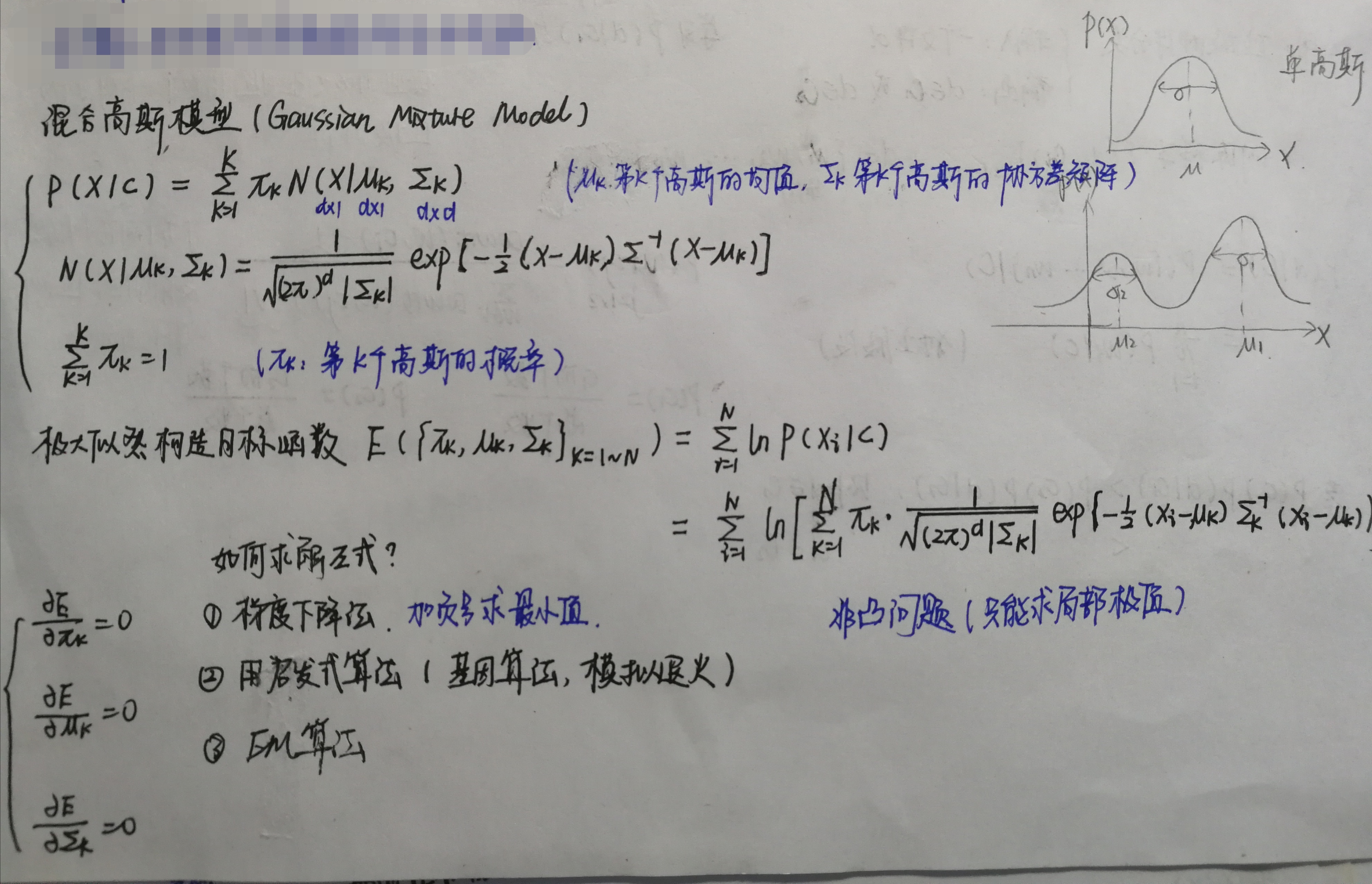
 1 def data_generator():
 2
 3     scale = 2.
 4     centers = [
 5         (1, 0),
 6         (-1, 0),
 7         (0, 1),
 8         (0, -1),
 9         (1. / np.sqrt(2), 1. / np.sqrt(2)),
10         (1. / np.sqrt(2), -1. / np.sqrt(2)),
11         (-1. / np.sqrt(2), 1. / np.sqrt(2)),
12         (-1. / np.sqrt(2), -1. / np.sqrt(2))
13     ]
14     centers = [(scale * x, scale * y) for x, y in centers]
15     while True:
16         dataset = []
17         for i in range(batchsz):
18             point = np.random.randn(2) * .02
19             center = random.choice(centers)
20
21             #N(0,1)sample出来一个点 + center_x1/x2
22             point[0] += center[0]
23             point[1] += center[1]
24             dataset.append(point)
25         dataset = np.array(dataset, dtype='float32')
26         dataset /= 1.414                                #stdev
27         yield dataset
5.可视化
 1 def generate_image(D, G, xr, epoch):      #xr表示真实的sample
 2     """
 3     Generates and saves a plot of the true distribution, the generator, and the
 4     critic.
 5     """
 6     N_POINTS = 128
 7     RANGE = 3
 8     plt.clf()
 9
10     points = np.zeros((N_POINTS, N_POINTS, 2), dtype='float32')
11     points[:, :, 0] = np.linspace(-RANGE, RANGE, N_POINTS)[:, None]
12     points[:, :, 1] = np.linspace(-RANGE, RANGE, N_POINTS)[None, :]
13     points = points.reshape((-1, 2))             # (16384, 2)
14
15
16     # draw contour
17     with torch.no_grad():
18         points = torch.Tensor(points)      # [16384, 2]
19         disc_map = D(points).cpu().numpy() # [16384]
20     x = y = np.linspace(-RANGE, RANGE, N_POINTS)
21     cs = plt.contour(x, y, disc_map.reshape((len(x), len(y))).transpose())
22     plt.clabel(cs, inline=1, fontsize=10)
23     # plt.colorbar()
24
25
26     # draw samples
27     with torch.no_grad():
28         z = torch.randn(batchsz, 2)                 # [b, 2]
29         samples = G(z).cpu().numpy()                # [b, 2]
30     plt.scatter(xr[:, 0], xr[:, 1], c='orange', marker='.')
31     plt.scatter(samples[:, 0], samples[:, 1], c='green', marker='+')
32
33     viz.matplot(plt, win='contour', opts=dict(title='p(x):%d'%epoch))
6.训练
和上面图片中的梯度上升法不同,下面训练使用的梯度下降法,所以对于原本需要最大化的的数据添加负号,就能实现梯度下降。
optim.Adam()中的batas参数用于计算梯度的平均和平方的系数(默认: (0.9, 0.999))
 1 def main():
 2
 3     torch.manual_seed(23)
 4     np.random.seed(23)
 5
 6     G = Generator()
 7     D = Discriminator()
 8     G.apply(weights_init)
 9     D.apply(weights_init)
10
11     optim_G = optim.Adam(G.parameters(), lr=1e-3, betas=(0.5, 0.9))
12     optim_D = optim.Adam(D.parameters(), lr=1e-3, betas=(0.5, 0.9))
13
14
15     data_iter = data_generator()
16     print('batch:', next(data_iter).shape)              #[b, 2]
17
18     viz.line([[0,0]], [0], win='loss', opts=dict(title='loss', legend=['D', 'G']))
19
20     for epoch in range(1000):
21
22         # 1. train discriminator for k steps
23         for _ in range(5):
24
25             #1.1首先train on real data
26             x = next(data_iter)
27             xr = torch.from_numpy(x)       #真实数据
28             predr = (D(xr))                # [b, 2] -> [b, 1]
29             # max log(lossr),即min (-lossr)
30             lossr = - (predr.mean())
31
32             #1.2 train on fake data
33             z = torch.randn(batchsz, 2)    # [b, 2]随机产生的伪数据
34             xf = G(z).detach()             # [b, 2] 此处固定G,更新D,所以不更新G的参数
35             predf = (D(xf))                # [b]
36             # min predf
37             lossf = (predf.mean())
38
39             loss_D = lossr + lossf
40
41             optim_D.zero_grad()
42             loss_D.backward()
43             optim_D.step()
44
45
46         # 2. train Generator
47         z = torch.randn(batchsz, 2)       #[b, 2]随机产生的伪数据
48         xf = G(z)
49         predf = (D(xf))
50         # max predf,即min(-predf)
51         loss_G = - (predf.mean())
52
53         optim_G.zero_grad()               #此处固定D,更新G,所以不更新D的参数
54         loss_G.backward()
55         optim_G.step()
56
57
58         if epoch % 100 == 0:
59             viz.line([[loss_D.item(), loss_G.item()]], [epoch], win='loss', update='append')
60             generate_image(D, G, xr, epoch)
61             print(loss_D.item(), loss_G.item())
62
63
64 if __name__ == '__main__':
65     main()
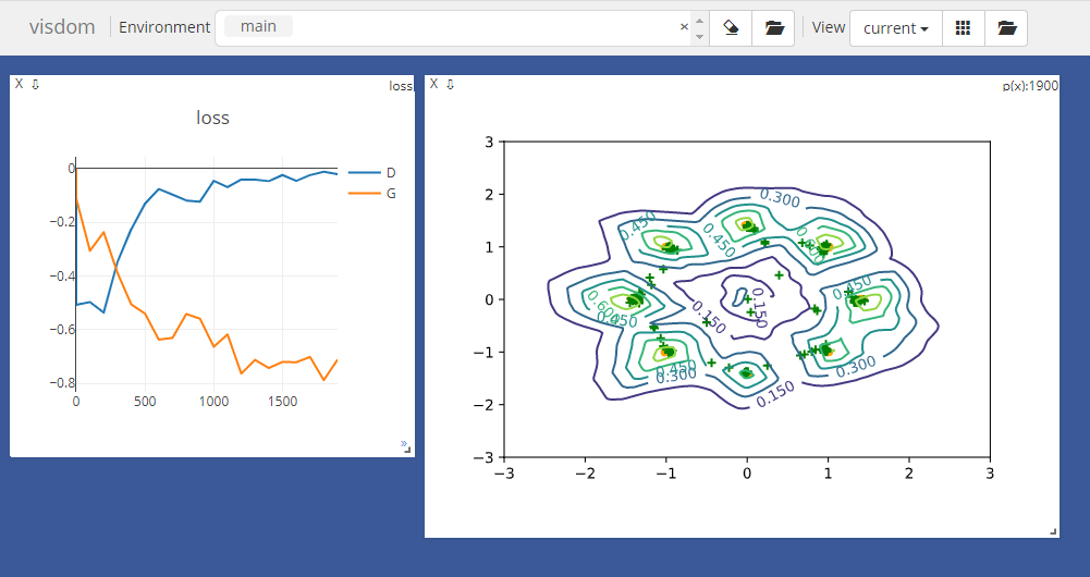
下图显示Generator和Discriminator的训练结果,两者的loss都接近于0,sample出来的数据经过Generator后覆盖住了真实数据。
 1 -0.6137181520462036 -0.0665668323636055
 2 7.620922672430937e-23 -6.780519236493468e-22
 3 2.8811570836759978e-37 -3.576674200342663e-41
 4 2.7326036398933606e-12 -5.0371435361452164e-33
 5 1.5811193901845998e-21 -1.796846778152569e-15
 6 2.1587619070328268e-20 -0.0
 7 2.0948376092776535e-32 -2.429269052203856e-16
 8 6.822592214491066e-14 -0.0
 9 9.122023851176224e-35 -2.9085079939065756e-34
10 0.0 -4.5381907731517276e-14

并不是每次运行都是这种结果,Generator常常由于GAN训练的不稳定(真实数据和生成数据没有重叠),loss保持在非0的某个值,长期得不到更新。
解决方案:W-GAN(通过用Wasserstein距离代替JS散度来优化训练的生成对抗网络)
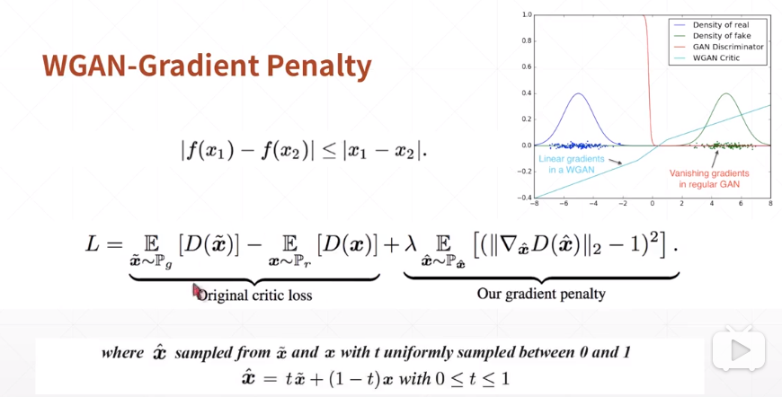
在代码中增加gradient penalty
 1 def gradient_penalty(D, xr, xf):  #xr和xf的shape=[b, 2]
 2
 3     t = torch.rand(batchsz, 1)   #sample一个均值分布[b, 1]
 4     t = t.expand_as(xr)          #[b, 1] -> [b, 2]
 5
 6     mid = t *xr +(1-t) * xf      #在真实数据和fake数据之间做线性差值,即图中的xhat
 7     mid.requires_grad_()         #设置导数信息
 8
 9     pred = D(mid)
10     grads = autograd.grad(outputs=pred, inputs=mid,
11                           grad_outputs=torch.ones_like(pred),
12                           create_graph=True, retain_graph=True, only_inputs=True)[0]     #create_graph用来二次求导
13
14     gp = torch.pow(grads.norm(2, dim=1) - 1, 2).mean()
15     return gp
在主函数中计算Discriminator的loss时加上gp项。
1             #1.3 gradient penalty
2             gp = gradient_penalty(D, xr, xf.detach())    #因为不需要对D求导,所以detach
3
4             loss_D = lossr + lossf + 0.2 * gp
迭代2000次的结果如下:
 1 -0.5074049830436707 -0.11114723235368729
 2 -0.4972265362739563 -0.3060861825942993
 3 -0.5360251665115356 -0.23698316514492035
 4 -0.3480537533760071 -0.3882521390914917
 5 -0.22527582943439484 -0.5057252645492554
 6 -0.13060471415519714 -0.5396959185600281
 7 -0.07626903057098389 -0.6366142630577087
 8 -0.09713903069496155 -0.6304153203964233
 9 -0.1190759465098381 -0.5412021279335022
10 -0.1230357214808464 -0.5588557124137878
11 -0.04560390114784241 -0.6632308959960938
12 -0.06906679272651672 -0.6173125505447388
13 -0.04104984924197197 -0.7628952860832214
14 -0.0408158078789711 -0.7121548652648926
15 -0.04687119275331497 -0.7424123287200928
16 -0.024066904559731483 -0.7196884751319885
17 -0.04576507583260536 -0.7208324670791626
18 -0.02462894842028618 -0.7012563943862915
19 -0.01230126153677702 -0.7875514030456543
20 -0.02122686244547367 -0.7108622193336487

 浙公网安备 33010602011771号