
梯度下降法
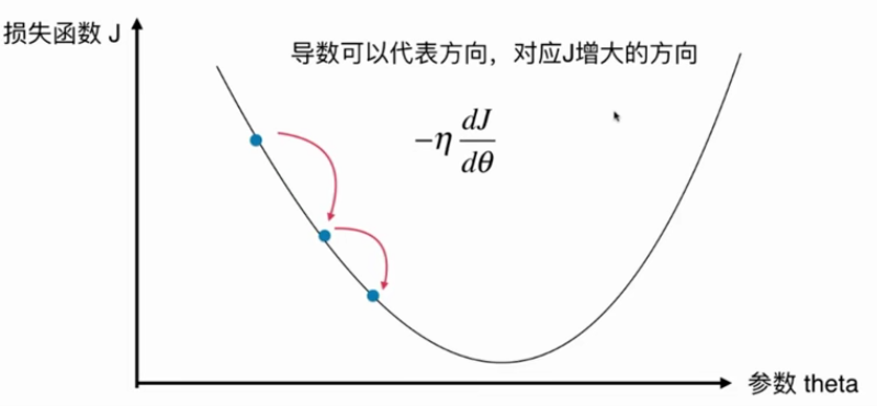
1.梯度下降法
是一种基于搜索的最优化方法,作用是最小化一个损失函数。
但不是所有的函数都有唯一的极值点。
解决方案:多次运行,随机初始化点
梯度下降法的初始点也是一个超参数
线性回归法的损失函数具有唯一的最优解。
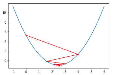
模拟实现梯度下降法
 1 import numpy as np
 2 import matplotlib.pyplot as plt
 3
 4 plot_x=np.linspace(-1, 6,141)
 5 plot_y=(plot_x-2.5)**2-1
 6
 7 def dJ(theta):
 8     return 2*(theta-2.5)
 9
10 def J(theta):
11     try:
12         return (theta-2.5)**2-1
13     except:
14         return float('inf')
15
16 #eta为学习速率,n_iters规定最大循环次数
17 def gradient_descent(initial_theta, eta, n_iters=1e4, epsilon=1e-8):
18
19     theta = initial_theta
20     theta_history.append(initial_theta)
21     i_iter=0                     #记录当前是第几次循环
22
23     while i_iter<n_iters:
24         gradient = dJ(theta)     #计算梯度
25         last_theta = theta       #更新theta
26         theta = theta - eta * gradient
27         theta_history.append(theta)
28
29         if (abs(J(theta) - J(last_theta)) < epsilon):
30             break
31
32         i_iter+=1
33
34 def plot_theta_history():
35     plt.plot(plot_x, J(plot_x))
36     plt.plot(np.array(theta_history),J(np.array(theta_history)),color='r',marker='+')
37     plt.show()
38
39 eta=0.1
40 theta_history=[]
41 gradient_descent(0, eta)
42 plot_theta_history()
当学习速率eta=0.1和eta=0.8时,相应的图像如下:

2.线性回归中的梯度下降法
因为多元线性回归的正规方程解复杂度较高,采用梯度下降法解决。
推导如下:
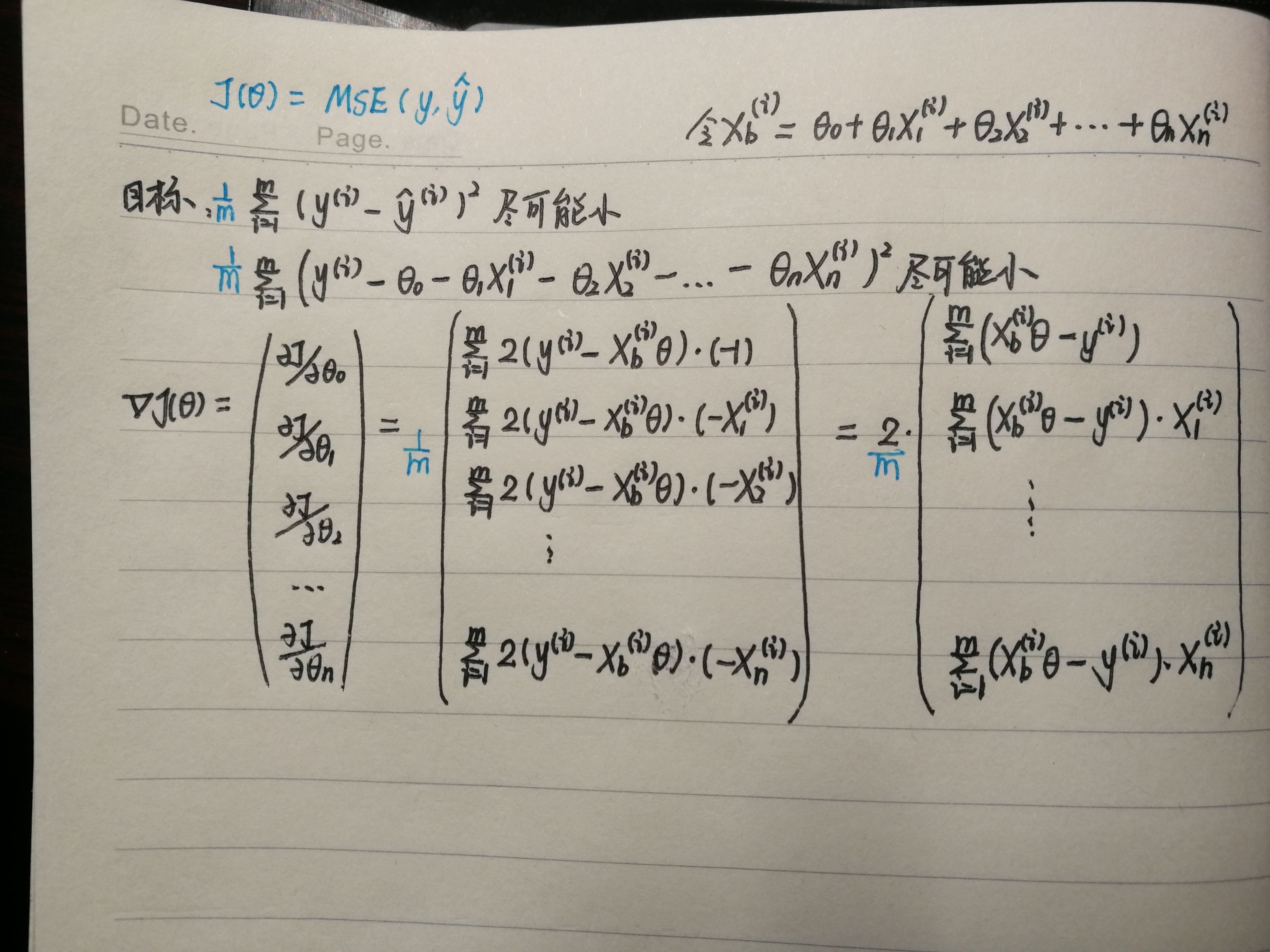
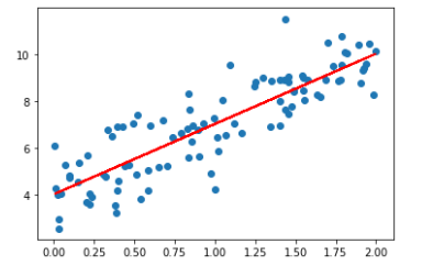
使用梯度下降法求解线性回归参数:
 1 import numpy as np
 2 import matplotlib.pyplot as plt
 3
 4 np.random.seed(666)
 5 x=2*np.random.random(size=100)
 6 y=x*3.+4.+np.random.normal(size=100) #(100,)
 7
 8 X=x.reshape(-1,1)    #(100,1)
 9
10 plt.scatter(x,y)
11
12 def J(theta,X_b,y):
13     try:
14         return np.sum((y-X_b.dot(theta))**2)/len(X_b)
15     except:
16         return float('inf')
17
18 def dJ(theta,X_b,y):
19     res=np.empty(len(theta))
20     res[0]=np.sum(X_b.dot(theta)-y)
21     for i in range(1,len(theta)):
22         res[i]=(X_b.dot(theta)-y).dot(X_b[:,i])
23
24     return res*2/len(X_b)
25
26 def gradient_descent(X_b, y, initial_theta, eta, n_iters=1e4, epsilon=1e-8):
27     theta = initial_theta
28     cur_iter = 0
29
30     while cur_iter < n_iters:
31         gradient = dJ(theta, X_b, y)
32         last_theta = theta
33         theta = theta - eta * gradient
34         if (abs(J(theta, X_b, y) - J(last_theta, X_b, y)) < epsilon):
35             break
36
37     cur_iter += 1
38     return theta
39
40 X_b=np.hstack([np.ones((len(X),1)),X])
41 initial_theta=np.zeros(X_b.shape[1])
42 eta=0.01
43
44 theta=gradient_descent(X_b, y, initial_theta, eta)
45 print(theta)      #对应截距和斜率(和调用LinearRegression中的fit函数拟合出的截距和斜率一致)
46
47 plt.plot(X,theta[0]+theta[1]*X)
48 plt.show()
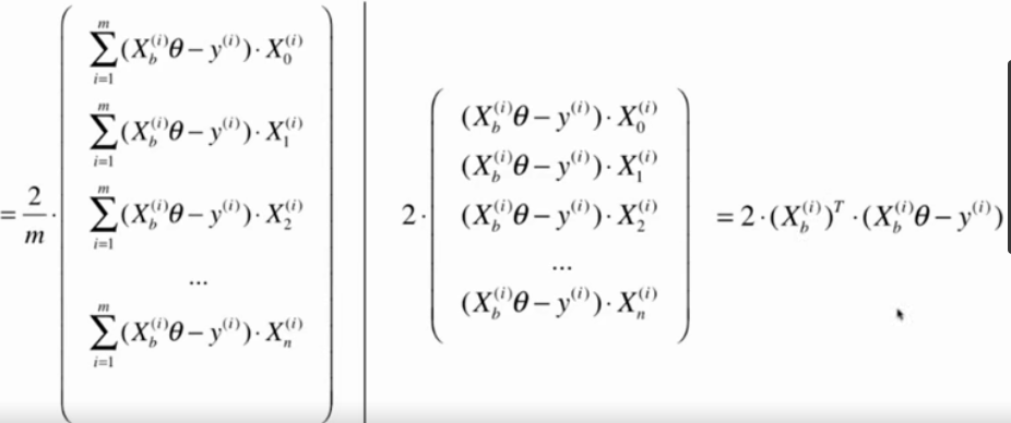
线性回归中梯度下降法的向量化
对上面的推导进行优化:

将上面for循环实现的dJ函数修改如下:
1 def dJ(theta,X_b,y):
2     return X_b.T.dot(X_b.dot(theta)-y)*2.0/len(X_b)
Tip:使用梯度下降之前要进行数据归一化。
3.随机梯度下降法
批量梯度下降法中,每一次计算过程都要将样本中所有信息进行批量计算,如果样本量很大,计算梯度就很耗时。于是引出随机梯度下降法,每次只取一行作为搜索的方向。
eta随着循环次数的增加,学习率降低。

手写随机梯度下降法
 1 import numpy as np
 2
 3 m=100000
 4 x=np.random.normal(size=m)
 5 X=x.reshape(-1,1)
 6 y=x*4.+3.+np.random.normal(0,3,size=m)
 7
 8 def dJ_sgd(theta,X_b_i,y_i):
 9     return X_b_i.T.dot(X_b_i.dot(theta)-y_i)*2.0
10
11 def sgd(X_b, y, initial_theta, n_iters):
12     t0=5
13     t1=50
14     def learning_rate(t):
15         return t0/(t+t1)
16
17     theta=initial_theta
18     for cur_iter in range(n_iters):
19         rand_i=np.random.randint(len(X_b))   #随机获得一个索引
20         gradient=dJ_sgd(theta, X_b[rand_i], y[rand_i])
21         theta=theta-learning_rate(cur_iter)*gradient
22     return theta
23
24 X_b=np.hstack([np.ones((len(X),1)),X])
25 initial_theta=np.zeros(X_b.shape[1])
26 eta=0.01
27
28 theta=sgd(X_b, y, initial_theta, n_iters=len(X_b)//3)   #只检测了三分之一个样本就可以达到比较好的结果
29 print(theta)      #对应截距和斜率
scikit-learn中的随机梯度下降法
 1 import numpy as np
 2 from sklearn import datasets
 3
 4 #波士顿房产数据
 5 boston=datasets.load_boston()
 6
 7 X=boston.data
 8 y=boston.target
 9
10 X=X[y<50.0]            #去除掉采集样本拥有的上限点
11 y=y[y<50.0]
12
13 #拆分数据集
14 from sklearn.model_selection import train_test_split
15 X_train,X_test,y_train,y_test=train_test_split(X,y,random_state=666)
16
17 #归一化处理
18 from sklearn.preprocessing import StandardScaler
19 standardScaler=StandardScaler()
20 standardScaler.fit(X_train)
21
22 X_train_standard=standardScaler.transform(X_train)
23 X_test_standard=standardScaler.transform(X_test)
24
25
26 from sklearn.linear_model import SGDRegressor
27 sgd_reg=SGDRegressor(n_iter_no_change=100)             #次数默认为5
28 sgd_reg.fit(X_train_standard,y_train)
29 print(sgd_reg.score(X_test_standard,y_test))
4.关于梯度的调试
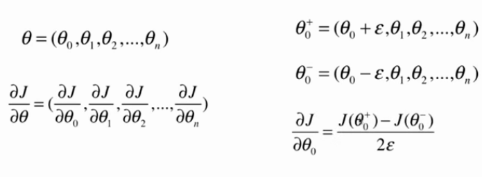
 1 import numpy as np
 2
 3 np.random.seed(666)
 4 X=np.random.random(size=(1000,10))
 5
 6 true_theta=np.arange(1,12,dtype=float)
 7
 8 X_b=np.hstack((np.ones((len(X),1)),X))
 9 y=X_b.dot(true_theta) + np.random.normal(size=1000)
10
11 def J(theta,X_b,y):
12     try:
13         return np.sum((y-X_b.dot(theta))**2)/len(X_b)
14     except:
15         return float('inf')
16
17 #只适用于当前损失函数J(相当于使用了求导公式,所以只适用于当前函数)
18 def dJ_math(theta,X_b,y):
19     return X_b.T.dot(X_b.dot(theta)-y)*2.0/len(y)
20
21 #适用于任何损失函数(相当于用定义求导,所以适用于任何函数)
22 def dJ_debug(theta,X_b,y,epsilon=0.01):
23     res=np.empty(len(theta))
24     for i in range(len(theta)):
25         theta_1=theta.copy()
26         theta_1[i]+=epsilon
27
28         theta_2=theta.copy()
29         theta_2[i]-=epsilon
30         res[i]=(J(theta_1,X_b,y)-J(theta_2,X_b,y))/(2*epsilon)
31     return res
32
33 def gradient_descent(dJ,X_b, y, initial_theta, eta, n_iters=1e4, epsilon=1e-8):
34     theta = initial_theta
35     cur_iter = 0
36
37     while cur_iter < n_iters:
38         gradient = dJ(theta, X_b, y)
39         last_theta = theta
40         theta = theta - eta * gradient
41         if (abs(J(theta, X_b, y) - J(last_theta, X_b, y)) < epsilon):
42             break
43
44     cur_iter += 1
45     return theta
46
47 initial_theta=np.zeros(X_b.shape[1])
48 eta=0.01
49 theta=gradient_descent(dJ_math, X_b, y, initial_theta, eta)
50 print(theta)
51
52 theta=gradient_descent(dJ_debug, X_b, y, initial_theta, eta)
53 print(theta)
dJ_debug方法比dJ_math方法要慢得多,通过这个方式可以先得到正确的结果,然后再推导公式求解梯度公式的数学解,最后将解和debug的解比较,从而判断我们推导的公式是否正确。

 浙公网安备 33010602011771号