

Android中的数据结构
数据结构在Android中也有着大量的运用,这里采用数据结构与源代码分析相结合,来认识Android的数据结构
线性表
线性表可分为顺序存储结构和链式存储结构
顺序存储结构-ArrayList
通过对源代码的产看得知,ArrayList继承自AbstractList,实现了多个接口,其中List里面就实现了常用的一些操作,包括增删改查清除大小等等
public class ArrayList<E> extends AbstractList<E>
        implements List<E>, RandomAccess, Cloneable, java.io.Serializable {
	···
}
ArrayList的实现其实就是基于数组,而且可以得知ArrayList的初始长度为10,数据进行了反序列化:transient
private static final int DEFAULT_CAPACITY = 10;
private static final Object[] EMPTY_ELEMENTDATA = {};
transient Object[] elementData;
private int size;
可以知道,ArrayList的数据初始化是在构造方法中完成的
public ArrayList(int initialCapacity) {
    super();
    if (initialCapacity < 0)
        throw new IllegalArgumentException("Illegal Capacity: "+
                                           initialCapacity);
    this.elementData = new Object[initialCapacity];
}

public ArrayList() {
    super();
    this.elementData = EMPTY_ELEMENTDATA;
}

public ArrayList(Collection<? extends E> c) {
    elementData = c.toArray();
    size = elementData.length;
    if (elementData.getClass() != Object[].class)
        elementData = Arrays.copyOf(elementData, size, Object[].class);
}
首先看一看add方法
public boolean add(E e) {
    ensureCapacityInternal(size + 1);  // Increments modCount!!
    elementData[size++] = e;
    return true;
}
这里的ensureCapacityInternal()方法比较重要,来看看这个方法都做了什么
private void ensureCapacityInternal(int minCapacity) {
    if (elementData == EMPTY_ELEMENTDATA) {
        minCapacity = Math.max(DEFAULT_CAPACITY, minCapacity);
    }

    ensureExplicitCapacity(minCapacity);
}
这里得到了最小需要的ArrayList大小,然后调用了ensureExplicitCapacity(),这里有一个modCount变量,用来记录元素的情况
private void ensureExplicitCapacity(int minCapacity) {
    modCount++;
    if (minCapacity - elementData.length > 0)
        grow(minCapacity);
}
这里做了判断,如果当前大小小于所需大小,那么就调用grow()方法,ArrayList之所以能到增长,其实现位置就在这里
private void grow(int minCapacity) {
    int oldCapacity = elementData.length;
    int newCapacity = oldCapacity + (oldCapacity >> 1);
    if (newCapacity - minCapacity < 0)
        newCapacity = minCapacity;
    if (newCapacity - MAX_ARRAY_SIZE > 0)
        newCapacity = hugeCapacity(minCapacity);
    elementData = Arrays.copyOf(elementData, newCapacity);
}
这里获取了元素的个数,然后计算新的个数,其增量是原个数的一半,然后得到其符合的值,如果需要的个数大于规定的最大值(Integer.MAX_VALUE - 8),那么就将其大小设置为Integer.MAX_VALUE或者Integer.MAX_VALUE - 8,
private static int hugeCapacity(int minCapacity) {
    if (minCapacity < 0) // overflow
        throw new OutOfMemoryError();
    return (minCapacity > MAX_ARRAY_SIZE) ?
        Integer.MAX_VALUE :
        MAX_ARRAY_SIZE;
}
到这里就已经将其长度增大了,再将原数据复制到新的数组,然后回到add方法,得知这时候将添加的元素放到之前最后面的位置elementData[size++] = e;,这样就实现了ArrayList数据的添加
其余方法和add方法类似,比如remove就是将元素置空,然后让GC去回收
public boolean remove(Object o) {
    if (o == null) {
        for (int index = 0; index < size; index++)
            if (elementData[index] == null) {
                fastRemove(index);
                return true;
            }
    } else {
        for (int index = 0; index < size; index++)
            if (o.equals(elementData[index])) {
                fastRemove(index);
                return true;
            }
    }
    return false;
}

private void fastRemove(int index) {
    modCount++;
    int numMoved = size - index - 1;
    if (numMoved > 0)
        System.arraycopy(elementData, index+1, elementData, index,
                         numMoved);
    elementData[--size] = null; // clear to let GC do its work
}
ArrayList的迭代器,用来遍历元素,迭代器里面的增加删除操作也和ArrayList的增加删除一样,需要对size进行操作
至此,ArrayList的简单解读就完成了
链式存储结构-LinkedList
在Android中的链式存储结构,就是使用双向链表实现的,有一个内部类Node,用来定义节点,初始化的时候是头节点指向尾节点,尾节点指向头节点
private static class Node<E> {
    E item;
    Node<E> next;
    Node<E> prev;

    Node(Node<E> prev, E element, Node<E> next) {
        this.item = element;
        this.next = next;
        this.prev = prev;
    }
}
其继承了AbstractSequentialList,并实现了一系列接口,可以看到不仅实现了List还实现了Deque双端队列
public class LinkedList<E> extends AbstractSequentialList<E>
    implements List<E>, Deque<E>, Cloneable, java.io.Serializable {
	···
}
定义的变量主要有三个,首节点,尾节点和大小
transient int size = 0;
transient Node<E> first;
transient Node<E> last;
首先依旧是查看add方法的操作
public boolean add(E e) {
    linkLast(e);
    return true;
}
这里调用了linkLast()方法,而这个方法是从尾部添加元素
void linkLast(E e) {
    final Node<E> l = last;
    final Node<E> newNode = new Node<>(l, e, null);
    last = newNode;
    if (l == null)
        first = newNode;
    else
        l.next = newNode;
    size++;
    modCount++;
}
还可以在指定位置添加元素,首先会检查添加位置是否合法,合法的意思就是index >= 0 && index <= size,如果插入的位置是末尾,那么就是尾插法,如果不是末尾,就调用linkBefore()
public void add(int index, E element) {
    checkPositionIndex(index);

    if (index == size)
        linkLast(element);
    else
        linkBefore(element, node(index));
}
会先调用node方法,得到指定位置的node,这里从中间开始查找,使得效率得到提高
这个思想在remove,set等里面都有使用到,这也是使用双向链表的原因,LinkedHashMap也是采用的双向链表
Node<E> node(int index) {
    // assert isElementIndex(index);

    if (index < (size >> 1)) {
        Node<E> x = first;
        for (int i = 0; i < index; i++)
            x = x.next;
        return x;
    } else {
        Node<E> x = last;
        for (int i = size - 1; i > index; i--)
            x = x.prev;
        return x;
    }
}
然后在指定node位置之前插入元素
void linkBefore(E e, Node<E> succ) {
    // assert succ != null;
    final Node<E> pred = succ.prev;
    final Node<E> newNode = new Node<>(pred, e, succ);
    succ.prev = newNode;
    if (pred == null)
        first = newNode;
    else
        pred.next = newNode;
    size++;
    modCount++;
}
其他的方法与add类似,主要就是后继和前驱的指向,以及插入位置的考量
ArrayList与LinkedList比较
ArrayList属于顺序存储,LinkedList属于链式存储
ArrayList的删除和插入效率低,查询效率高,而LinkedList则刚好相反
在实际使用中要根据具体使用情况选择
栈和队列
栈和队列是两种不同读取方式的数据结构,栈属于先进后出,而队列属于先进先出,要比喻的话,栈好比一个瓶子,先放进去的要最后才能取出来,队列还比就是一根管子,先进去的先出来,在Android中有着这两种数据结构思想的实现类
栈
这里就是Stack这个类,由于代码不多,直接全部贴出来
public
class Stack<E> extends Vector<E> {

    public Stack() {
    }

    public E push(E item) {
        addElement(item);

        return item;
    }

    public synchronized E pop() {
        E       obj;
        int     len = size();

        obj = peek();
        removeElementAt(len - 1);

        return obj;
    }

    public synchronized E peek() {
        int     len = size();

        if (len == 0)
            throw new EmptyStackException();
        return elementAt(len - 1);
    }

    public boolean empty() {
        return size() == 0;
    }

    public synchronized int search(Object o) {
        int i = lastIndexOf(o);

        if (i >= 0) {
            return size() - i;
        }
        return -1;
    }

    private static final long serialVersionUID = 1224463164541339165L;
}
可以看到有push(),pop(),peek(),empty(),search()方法,其中pop和peek的区别在于前者会删除元素,而后者不会,后者只是查看元素,那么其具体实现是怎么样的呢,这就在其父类Vextor中有所体现,查看源代码,其实和ArrayList基本上是一致的,无论是思想还是实现,在细微处有小区别,Vextor的扩容方式允许单个扩容,所以说Android中的栈实现是基于顺序链表的,push是添加元素,search是查找元素,从栈顶向栈底查找,一旦找到返回位置,pop和peek都是查看元素
另外,LinkedList也实现了栈结构
public void push(E e) {
    addFirst(e);
}
而addFirst()则是调用了linkFirst()方法,也就是采用了头插法
public void addFirst(E e) {
    linkFirst(e);
}
那么pop也应该是使用头部删除,果不其然
public E pop() {
    return removeFirst();
}
队列
队列也分为顺序结构实现和链式结构实现,但前者由于出队复杂度高0(n),容易假溢出,虽然可以通过首尾相连解决假溢出,这也就是循环队列,但实际中,基本是使用链式存储实现的,有一个接口就是队列的模型
public interface Queue<E> extends Collection<E> {
    boolean add(E e);
    boolean offer(E e);
    E remove();
    E poll();
    E element();
    E peek();
}
而在LinkedList实现了Deque接口,而Deque又是Queue的子类,故而之前的分析已经包含了队列
那么这次聚焦在Queue上,看看其都多是怎么做的
前面的分析我们已经知道了add方法调用的是linkLast(),也就是使用尾插法,那么offer方法呢
public boolean offer(E e) {
    return add(e);
}
可以看到offer()调用了add(),再看看剩下的方法,主要是remove方法
public E remove() {
    return removeFirst();
}
移除的是首位置,而添加的是尾(与队列队尾插入一致)
public E poll() {
    final Node<E> f = first;
    return (f == null) ? null : unlinkFirst(f);
}
public E peek() {
    final Node<E> f = first;
    return (f == null) ? null : f.item;
}
poll返回的也是首位置,peek也是(与队列队头取出一致)
public E element() {
    return getFirst();
}
element()返回首节点
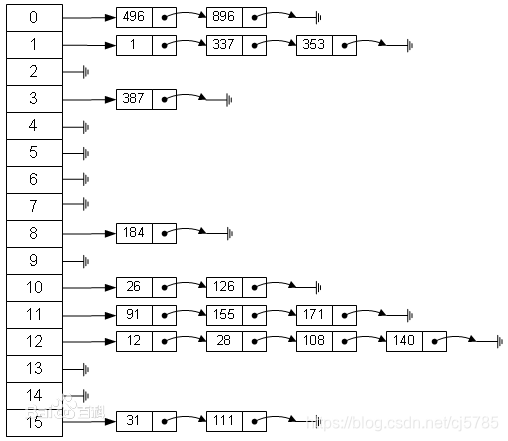
HashMap与LinkedHashMap
这两个严格来说不算数据结构,这里将其提取出来,是因为这两个在Android中有着广泛运用
HashMap
首先看一下继承类和实现接口,AbstractMap实现了Map里面的绝大部分方法,只有eq没有实现
public class HashMap<K,V> extends AbstractMap<K,V>
    implements Map<K,V>, Cloneable, Serializable {
	···
}
大概看一下其结构,依旧是扫一眼内部类,其主要包括以下四类
HashMapEntry:一个个的键值对,其在Android中为hide,提供了包括Key的获取,Value的设置获取,比较等方法,注意这是一个节点,也就是说这也是通过链表组织起来的,不过这个链表属于散列链表
XxxIterator:HashIterator,ValueIterator,KeyIterator,EntryIterator,今三个迭代器继承自第一个,用来获取相应的值
XxxSpliterator:HashMapSpliterator,KeySpliterator,ValueSpliterator,EntrySpliterator
XxxSet:KeySet,EntrySet,另外Value类也与其类似,不过没有使用Set,这也就是为何value可以重复而key不能重复的原因,这是用来记录值的集合
大致知道内部类的功能及其作用以后,就该看一看其成员变量了
static final int DEFAULT_INITIAL_CAPACITY = 4;
static final int MAXIMUM_CAPACITY = 1 << 30;
static final float DEFAULT_LOAD_FACTOR = 0.75f;
static final HashMapEntry<?,?>[] EMPTY_TABLE = {};
transient HashMapEntry<K,V>[] table = (HashMapEntry<K,V>[]) EMPTY_TABLE;
transient int size;
int threshold;
final float loadFactor = DEFAULT_LOAD_FACTOR;
transient int modCount;
首先是初始化大小为4,也就是说HashMap自创建开始就有4的容量,其最大容量为230,默认增长系数为0.75,也就是说其存储容量达到总容量的75%时候,会自动扩容另外还定义了键值对,大小等
那么接下来轮到构造方法了
public HashMap(int initialCapacity, float loadFactor) {
    if (initialCapacity < 0)
        throw new IllegalArgumentException("Illegal initial capacity: " +
                                           initialCapacity);
    if (initialCapacity > MAXIMUM_CAPACITY) {
        initialCapacity = MAXIMUM_CAPACITY;
    } else if (initialCapacity < DEFAULT_INITIAL_CAPACITY) {
        initialCapacity = DEFAULT_INITIAL_CAPACITY;
    }

    if (loadFactor <= 0 || Float.isNaN(loadFactor))
        throw new IllegalArgumentException("Illegal load factor: " +
                                           loadFactor);
    threshold = initialCapacity;
    init();
}

public HashMap(int initialCapacity) {
    this(initialCapacity, DEFAULT_LOAD_FACTOR);
}

public HashMap() {
    this(DEFAULT_INITIAL_CAPACITY, DEFAULT_LOAD_FACTOR);
}

public HashMap(Map<? extends K, ? extends V> m) {
    this(Math.max((int) (m.size() / DEFAULT_LOAD_FACTOR) + 1,
                  DEFAULT_INITIAL_CAPACITY), DEFAULT_LOAD_FACTOR);
    inflateTable(threshold);

    putAllForCreate(m);
}
简单来说就是将设置的成员变量初始化,这里的init()为一个空方法
与上面分析线性表的思路一样,我们先看添加元素的方法put()
public V put(K key, V value) {
    if (table == EMPTY_TABLE) {
        inflateTable(threshold);
    }
    if (key == null)
        return putForNullKey(value);
    int hash = sun.misc.Hashing.singleWordWangJenkinsHash(key);
    int i = indexFor(hash, table.length);
    for (HashMapEntry<K,V> e = table[i]; e != null; e = e.next) {
        Object k;
        if (e.hash == hash && ((k = e.key) == key || key.equals(k))) {
            V oldValue = e.value;
            e.value = value;
            e.recordAccess(this);
            return oldValue;
        }
    }

    modCount++;
    addEntry(hash, key, value, i);
    return null;
}
我们来详细分析一下在这里面到底做了啥,首先要保证table不为空,然后如果key为空,那么就存储NullKey的value,那么这是怎么操作的呢,在putForNullKey()我们可以看到,这里使用了addEntry(0, null, value, 0);,也就是说在HashMap里面是可以存null键的,不过最多只能存一个,后面的会覆盖掉前面的,就下来计算了hash值,在indexFor()里面就一句话return h & (length-1);,这里是获取到其索引值,这个索引值用来建立散列表的索引,关于散列表,使用一张百度百科的图来说明
for循环里面,会遍历整个table,如果hash值和key都相同,那么会覆盖之前的key,并返回那个key所对应的值,也就是说此时是没有添加成功的,那么在hash值不等或者key不等的情况下,会调用addEntry()方法,向散列表中添加,然后返回null
那么在addEntry()里面也就是添加元素的方法了
void addEntry(int hash, K key, V value, int bucketIndex) {
    if ((size >= threshold) && (null != table[bucketIndex])) {
        resize(2 * table.length);
        hash = (null != key) ? sun.misc.Hashing.singleWordWangJenkinsHash(key) : 0;
        bucketIndex = indexFor(hash, table.length);
    }

    createEntry(hash, key, value, bucketIndex);
}
在这里,计算了大小,如果容量不足,那么容量变为原来的两倍,也就是说HashMap的大小为2的整次幂,同时重新计算hash和index,那么接下来就是真正添加元素的地方了
那么我们继续看元素是怎么被添加的吧
void createEntry(int hash, K key, V value, int bucketIndex) {
    HashMapEntry<K,V> e = table[bucketIndex];
    table[bucketIndex] = new HashMapEntry<>(hash, key, value, e);
    size++;
}
这里传入新值,并且完成了链表的指向,增加了size的大小,整个添加的流程就完成了
这是插在数组元素位置的,后面连接起来
接下来看一看get()方法
public V get(Object key) {
    if (key == null)
        return getForNullKey();
    Entry<K,V> entry = getEntry(key);

    return null == entry ? null : entry.getValue();
}
这里可以看出,可以取key为null的value,然后调用getEntry()查找Entry
final Entry<K,V> getEntry(Object key) {
    if (size == 0) {
        return null;
    }

    int hash = (key == null) ? 0 : sun.misc.Hashing.singleWordWangJenkinsHash(key);
    for (HashMapEntry<K,V> e = table[indexFor(hash, table.length)];
         e != null;
         e = e.next) {
        Object k;
        if (e.hash == hash &&
            ((k = e.key) == key || (key != null && key.equals(k))))
            return e;
    }
    return null;
}
这里根据key计算出hash,然后再计算出index,去响应的table查找匹配的HashMapEntry,找到则返回,没找到返回空
然后判断entry是否为null,为null返回null,不为空则返回value值
LinkedHashMap
LruCache类使用到了LinkedHashMap,那么LinkedHashMap是怎么实现知道新旧添加的元素的呢
LinkedHashMap本身继承了HashMap,但是在数据结构上稍有不同,HashMap使用的是散列单向链表,而LinkedHashMap使用的是散列双向循环链表
private static class LinkedHashMapEntry<K,V> extends HashMapEntry<K,V> {
    LinkedHashMapEntry<K,V> before, after;

    LinkedHashMapEntry(int hash, K key, V value, HashMapEntry<K,V> next) {
        super(hash, key, value, next);
    }

    private void remove() {
        before.after = after;
        after.before = before;
    }

    private void addBefore(LinkedHashMapEntry<K,V> existingEntry) {
        after  = existingEntry;
        before = existingEntry.before;
        before.after = this;
        after.before = this;
    }

    void recordAccess(HashMap<K,V> m) {
        LinkedHashMap<K,V> lm = (LinkedHashMap<K,V>)m;
        if (lm.accessOrder) {
            lm.modCount++;
            remove();
            addBefore(lm.header);
        }
    }

    void recordRemoval(HashMap<K,V> m) {
        remove();
    }
}
这里主要看get()方法
public V get(Object key) {
    LinkedHashMapEntry<K,V> e = (LinkedHashMapEntry<K,V>)getEntry(key);
    if (e == null)
        return null;
    e.recordAccess(this);
    return e.value;
}
注意到这里调用了recordAccess(),而这个方法的实现就比较有意思了
void recordAccess(HashMap<K,V> m) {
    LinkedHashMap<K,V> lm = (LinkedHashMap<K,V>)m;
    if (lm.accessOrder) {
        lm.modCount++;
        remove();
        addBefore(lm.header);
    }
}
这里的if判断条件,我们回到LruCache,发现在给map初始化的时候,传递的参数为new LinkedHashMap<K, V>(0, 0.75f, true),也就是说这里的accessOrder为真,真的意思就是要按照新旧排序,这里调用了remove,那么在remove里面做了啥呢
private void remove() {
    before.after = after;
    after.before = before;
}
可以看到,在这个方法里面就是将当前元素断链了
然后还调用了addBefore()方法,这又是为何
private void addBefore(LinkedHashMapEntry<K,V> existingEntry) {
    after  = existingEntry;
    before = existingEntry.before;
    before.after = this;
    after.before = this;
}
这里将断链的节点放到最末尾,然后和头节点连起来了,那么这样每次get()的元素都会到最末尾,header的after就是最老的和最不常用的节点了,在LruCache自动释放内存时就是从这开始释放的,保证常用常驻
那么接下来再看看put方法,这里可以看到只是继承了HashMap的get方法,那么在哪里修改添加的呢
void addEntry(int hash, K key, V value, int bucketIndex) {
	LinkedHashMapEntry<K,V> eldest = header.after;
    if (eldest != header) {
        boolean removeEldest;
        size++;
        try {
            removeEldest = removeEldestEntry(eldest);
        } finally {
            size--;
        }
        if (removeEldest) {
            removeEntryForKey(eldest.key);
        }
    }

    super.addEntry(hash, key, value, bucketIndex);
}
可以看见这里重写了addEntry()方法,但里面并没有具体的创建,在这里的removeEldestEntry()也是直接返回false了
所以又重写了createEntry()
void createEntry(int hash, K key, V value, int bucketIndex) {
    HashMapEntry<K,V> old = table[bucketIndex];
    LinkedHashMapEntry<K,V> e = new LinkedHashMapEntry<>(hash, key, value, old);
    table[bucketIndex] = e;
    e.addBefore(header);
    size++;
}
可以看到这里也调用了addBefore(),也是加在了最后面,也就与header.before连接起来了
综合分析得出结论:LinkedHashMap不断调整元素位置,使得header.after为最不常用或者最先加入的元素,方便删除的时候直接移除
树
树当中,研究最多的就是二叉树
二叉树
二叉树的性质:
性质1:在二叉树的第i层上至多有2i-1个结点(i>=1)
性质2:深度为k的二叉树至多有2k-1个结点(k>=1)
性质3:对任何一颗二叉树T,如果其终端结点数为n0,度为2的结点数为n2,则n0 = n2+1
性质4:具有n个结点的完全二叉树深度为[log2n]+1 ([x]表示不大于x的最大整数)
性质5:如果对一颗有n个结点的完全二叉树(其深度为[log2(n+1)])的结点按层序编号(从第1层到第[log2(n+1)]层,每层从左到右),对任意一个结点i(1<=i<=n)有:
1).如果i=1,则结点i是二叉树的根,无双亲;如果i>1,则其双亲是结点[i/2]
2).如果2i>n,则结点i无左孩子(结点i为叶子结点);否则其左孩子是结点2i
3).如果2i+1>n,则结点i无右孩子;否则其右孩子是结点2i+1
二叉树高度和节点数
- 二叉树的高度
public int getHeight(){
	return getHeight(root);
}
private int getHeight(TreeNode node) {
	if(node == null){
		return 0;
	}else{
		int i = getHeight(node.leftChild);
		int j = getHeight(node.rightChild);
		return (i < j) ? j + 1 : i + 1;
	}
}
- 二叉树的结点数
public int getSize(){
	return getSize(root);
}
private int getSize(TreeNode node) {
	if(node == null){
		return 0;
	}else{
		return 1 + getSize(node.leftChild) + getSize(node.rightChild);
	}
}
二叉树的遍历
- 前序遍历
规则是若二叉树为空,则空操作返回,否则先访问跟结点,然后前序遍历左子树,再前序遍历右子树
public void preOrder(TreeNode node){
	if(node == null){
		return;
	}else{
		System.out.println("preOrder data:" + node.getData());
		preOrder(node.leftChild);
		preOrder(node.rightChild);
	}
}
- 中序遍历
规则是若树为空,则空操作返回,否则从根结点开始(注意并不是先访问根结点),中序遍历根结点的左子树,然后是访问根结点,最后中序遍历右子树
public void midOrder(TreeNode node){
	if(node == null){
		return;
	}else{
		midOrder(node.leftChild);
		System.out.println("midOrder data:" + node.getData());
		midOrder(node.rightChild);
	}
}
- 后序遍历
规则是若树为空,则空操作返回,否则从左到右先叶子后结点的方式遍历访问左右子树,最后是访问根结点
public void postOrder(TreeNode node){
	if(node == null){
		return;
	}else{
		postOrder(node.leftChild);
		postOrder(node.rightChild);
		System.out.println("postOrder data:" + node.getData());
	}
}
- 层序遍历
规则是若树为空,则空操作返回,否则从树的第一层,也就是根结点开始访问,从上而下逐层遍历,在同一层,按从左到右的顺序对结点逐个访问
生成二叉树
public TreeNode createBinaryTree(int size, ArrayList<String> datas) {
	if(datas.size() == 0) {
		return null;
	}
	String data = datas.get(0);
	TreeNode node;
	int index = size - datas.size();
	if(data.equals("#")) {
		node = null;
		datas.remove(0);
		return node;
	}
	node = new TreeNode(index, data);
	if(index == 0) {
		root = node;
	}
	datas.remove(0);
	node.leftChild = createBinaryTree(size, datas);
	node.rightChild = createBinaryTree(size, datas);
	return node;
}
查找二叉树(搜索二叉树)
在二叉树中,左节点小于根节点,有节点大于根节点的的二叉树成为查找二叉树,也叫做搜索二叉树
public class SearchBinaryTree {

	public static void main(String[] args) {
		SearchBinaryTree tree = new SearchBinaryTree();
		int[] intArray = new int[] {50, 27, 30, 60, 20, 40};
		for (int i = 0; i < intArray.length; i++) {
			tree.putTreeNode(intArray[i]);
		}
		tree.midOrder(root);
	}

	private static TreeNode root;
	public SearchBinaryTree() {}

	//创建查找二叉树,添加节点
	public TreeNode putTreeNode(int data) {
		TreeNode node = null;
		TreeNode parent = null;
		if (root == null) {
			node = new TreeNode(0, data);
			root = node;
			return root;
		}
		node = root;
		while(node != null) {
			parent = node;
			if(data > node.data) {
				node = node.rightChild;
			}else if(data < node.data) {
				node = node.leftChild;
			}else {
				return node;
			}
		}
		//将节点添加到相应位置
		node = new TreeNode(0, data);
		if(data < parent.data) {
			parent.leftChild = node;
		}else {
			parent.rightChild = node;
		}
		node.parent = parent;
		return root;
	}

	//验证是否正确
	public void midOrder(TreeNode node){
		if(node == null){
			return;
		} else {
			midOrder(node.leftChild);
			System.out.println("midOrder data:" + node.getData());
			midOrder(node.rightChild);
		}
	}

	class TreeNode{
		private int key;
		private int data;
		private TreeNode leftChild;
		private TreeNode rightChild;
		private TreeNode parent;
		public TreeNode(int key, int data) {
			super();
			this.key = key;
			this.data = data;
			leftChild = null;
			rightChild = null;
			parent = null;
		}
		public int getKey() {
			return key;
		}
		public void setKey(int key) {
			this.key = key;
		}
		public int getData() {
			return data;
		}
		public void setData(int data) {
			this.data = data;
		}
		public TreeNode getLeftChild() {
			return leftChild;
		}
		public void setLeftChild(TreeNode leftChild) {
			this.leftChild = leftChild;
		}
		public TreeNode getRightChild() {
			return rightChild;
		}
		public void setRightChild(TreeNode rightChild) {
			this.rightChild = rightChild;
		}
		public TreeNode getParent() {
			return parent;
		}
		public void setParent(TreeNode parent) {
			this.parent = parent;
		}
	}
}
删除节点
//删除节点
public void deleteNode(int key) throws Exception {
	TreeNode node = searchNode(key);
	if(node == null) {
		throw new Exception("can not find node");
	}else {
		delete(node);
	}
}

private void delete(TreeNode node) throws Exception {
	if(node == null) {
		throw new Exception("node is null");
	}
	TreeNode parent = node.parent;
	//删除的节点无左右节点
	if(node.leftChild == null && node.rightChild == null) {
		if(parent.leftChild == node) {
			parent.leftChild = null;
		}else {
			parent.rightChild = null;
		}
		return;
	}
	//被删除的节点有左节点无右节点
	if(node.leftChild != null && node.rightChild == null) {
		if(parent.leftChild == node) {
			parent.leftChild = node.leftChild;
		}else {
			parent.rightChild = node.leftChild;
		}
		return;
	}
	//被删除的节点无左节点有右节点
	if(node.leftChild == null && node.rightChild != null) {
		if(parent.leftChild == node) {
			parent.leftChild = node.rightChild;
		}else {
			parent.rightChild = node.rightChild;
		}
		return;
	}
	//被删除节点既有左结点又有右节点
	TreeNode next = getNextNode(node);
	delete(next);
	node.data = next.data;
}

private TreeNode getNextNode(TreeNode node) {
	if(node == null) {
		return null;
	}
	if(node.rightChild != null) {
		return getMinTreeNode(node.rightChild);
	}else {
		TreeNode parent = node.parent;
		while(parent != null && node == parent.rightChild) {
			node = parent;
			parent = parent.parent;
		}
		return parent;
	}
}

//找某节点的最小关键节点
private TreeNode getMinTreeNode(TreeNode node) {
	if(node == null) {
		return null;
	}
	while(node.leftChild != null) {
		node = node.leftChild;
	}
	return node;
}

private TreeNode searchNode(int key) {
	TreeNode node = root;
	if(node == null) {
		return null;
	}
	while(node != null && key != node.data) {
		if(key < node.data) {
			node = node.leftChild;
		}else {
			node = node.rightChild;
		}
	}
	return node;
}
图
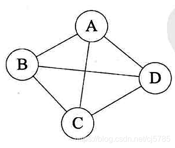
图(Graph)是由顶点的有穷非空集合和顶点之间边的集合组成,通常表示为:G(V,E),其中G表示一个图,V是图G中定点的集合,E是图G中边的集合
图中的数据元素称之为顶点,任意两个顶点之间都可能有关系,顶点之间的逻辑关系用边来表示,边集可以为空
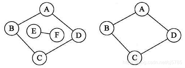
无向图和有向图
- 无向图
无向边:若顶点vi到vj之间的边没有方向,则称这条边为无向边(Edge),用无序偶对(vi,vj)来表示,如果图中任意两个顶点之间的边都是无向边,则称该图为无向图(Undirected Graphs)
在无向图中,如果任意两个顶点之间的边都存在,那么该图称为无向完全图
![Android中的数据结构-无向图]()
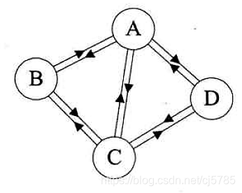
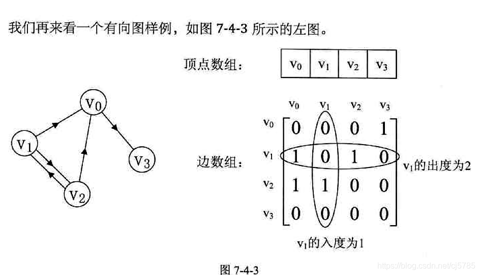
- 有向图
有向边:若顶点vi到vj的边有方向,则称这条边为有向边,也称之为弧(Arc),用有序偶对<vi,vj>来表示,如果图中任意两个顶点之间的边都是有向边,则称该图为有向图(Directed Graphs)
在有向图中,如果任意两个顶点之间都存在方向互为相反的两条弧,那么该图称为有向完全图
![Android中的数据结构-有向图]()
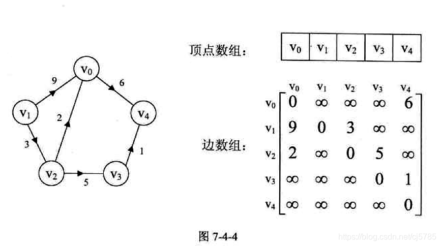
图的权
有些图的边或者弧具有与他相关的数字,这种与图的边或弧相关的数叫做权
连通图
在无向图G中,如果从顶点v到顶点v’有路径,则称v和v’是连通的,如果对于图中任意两个顶点vi,vj∈E,vi和vj都是连通的,则称G是连通图(Connected Graph)
度
无向图顶点的边数叫度,有向图顶点的边数叫出度和入度
图的存储结构
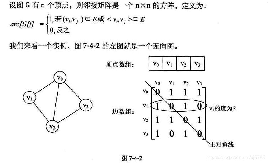
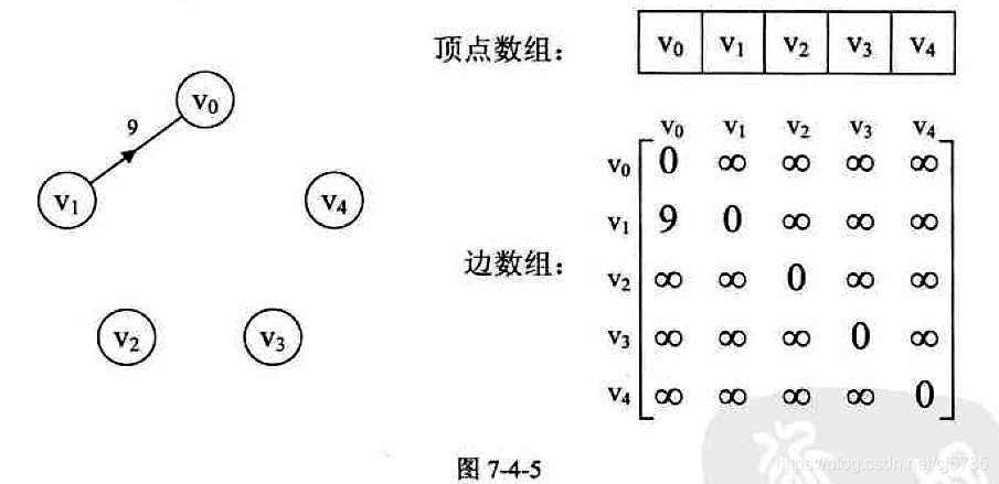
邻接矩阵
图的邻接矩阵(Adjacency Matrix)存储方式是用两个数组来表示图,一个一维数组存储图中的顶点信息,一个二维数组(称为邻接矩阵)存储图中的-边或弧信息
- 邻接矩阵
![Android中的数据结构-邻接矩阵1]()
![Android中的数据结构-邻接矩阵2]()
- 带权邻接矩阵
![Android中的数据结构-邻接矩阵3]()
- 浪费的邻接矩阵
![Android中的数据结构-邻接矩阵4]()
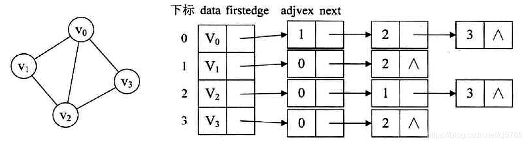
邻接表
讲到了一种孩子表示法,将结点存入数组,并对结点的孩子进行链式存储,不管有多少孩子,也不会存在空间浪费问题,这个思路同样适用于图的存储。我们把这种数组与链表相结合的存储方法称为邻接表
- 无向图的邻接表:
![Android中的数据结构-无向图邻接表]()
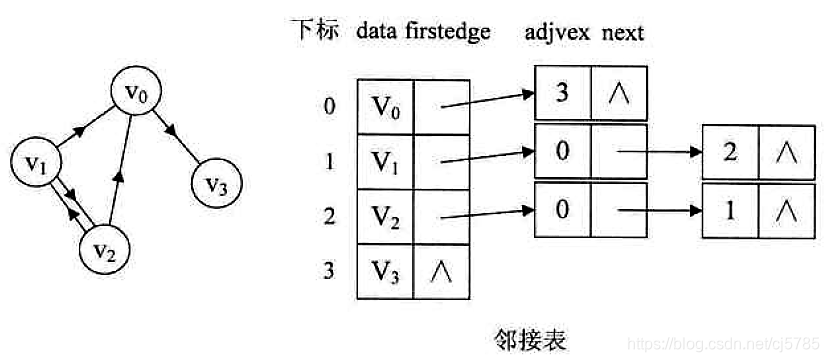
- 有向图的邻接表:
![Android中的数据结构-有向图的邻接表]()
- 有向图的逆邻接表
![Android中的数据结构-有向图的逆邻接表]()
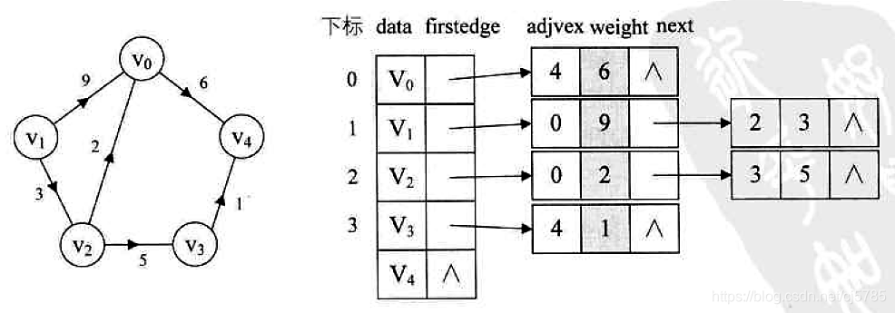
- 带权值邻接表
![Android中的数据结构-带权值邻接表]()

邻接矩阵的代码实现(Java)
public class Graph {
	private int vertexSize; //顶点数量
	private int[] vertexs; //顶点数组
	private int[][] matrix; //边数组
	private static final int MAX_WEIGHT = 1000; //非连接顶点权值

	public Graph(int vertexSize) {
		this.vertexSize = vertexSize;
		this.vertexs = new int[vertexSize];
		this.matrix = new int[vertexSize][vertexSize];
		//顶点初始化
		for (int i = 0; i < vertexSize; i++) {
			vertexs[i]= i;
		}
	}

	//计算某顶点出度
	public int getOutDegree(int index) {
		int degree = 0;
		for (int i = 0; i < matrix[index].length; i++) {
			int weight = matrix[index][i];
			if(weight != 0 && weight != MAX_WEIGHT) {
				degree++;
			}
		}
		return degree;
	}

	//获取两顶点之间的权值
	public int getWeight(int v1, int v2) {
		int weight = matrix[v1][v2];
		return weight == 0 ? 0 : (weight == MAX_WEIGHT ? -1 : weight);
	}

	public static void main(String[] args) {
		Graph graph = new Graph(5);
		int[] a1 = new int[] {0,MAX_WEIGHT,MAX_WEIGHT,MAX_WEIGHT,6};
		int[] a2 = new int[] {9,0,3,MAX_WEIGHT,MAX_WEIGHT};
		int[] a3 = new int[] {2,MAX_WEIGHT,0,5,MAX_WEIGHT};
		int[] a4 = new int[] {MAX_WEIGHT,MAX_WEIGHT,MAX_WEIGHT,0,1};
		int[] a5 = new int[] {MAX_WEIGHT,MAX_WEIGHT,MAX_WEIGHT,MAX_WEIGHT,0};
		graph.matrix[0] = a1;
		graph.matrix[1] = a2;
		graph.matrix[2] = a3;
		graph.matrix[3] = a4;
		graph.matrix[4] = a5;
		int degree = graph.getOutDegree(0);
		int weight = graph.getWeight(2, 0);
		System.out.println("degree:" + degree);
		System.out.println("weight:" + weight);
	}
}
图的遍历
图的遍历和树的遍历类似,从某一顶点出发遍历图中其余顶点,且使得每个顶点有且只有一次访问,这一过程叫做图的遍历
深度优先遍历
深度优先遍历(Depth_First_Search),也称为深度优先搜素,简称DFS
他从图中某个顶点v出发,访问此顶点,然后从v的未被访问的邻接点出发深度优先遍历图,直到图中所有和v有路径相通的顶点都被访问到
下面是深度优先遍历的伪代码©
typedef int Boolean;
Boolean visited[Max];
void DFS(MGraph G,int i){
	int j;
	visited[i] = TRUE;
	printf("%c", G.vexs[i]);
	for(j = 0; j < G.numVertexes; j++){
		if(G.arc[i][j] == 1&&!visited[j]){
			DFS(G,j);
		}
	}
}
void DFSTraverse(MGraph G){
	int i;
	for(i = 0 ;i<G.numVertexes;i++){
		visited[i] = FALSE;
	}
	for(i = 0; i < G.numVertexes; i++){
		if(!visited[i]){
			DFS(G,i);
		}
	}
}
有了思路就可以写出Java代码了
private boolean[] isVisited; //是否遍历过

//获取某个顶点的连接点:其实就是遍历一行,获取不为零且不为MAX_WEIGHT的第一个位置
public int getFirstNeighbor(int v) {
	for (int j = 0; j < vertexSize; j++) {
		if(matrix[v][j] > 0 && matrix[v][j] < MAX_WEIGHT) {
			return j;
		}
	}
	return -1;
}

//根据前一个邻接点的下标获得下一个邻接点:就是找到一行中第二个有意义的位置
//v代表要找的顶点,也就是要找的那一行,index代表从这个位置往后开始找
private int getNextNeighbor(int v, int index) {
	for (int j = index + 1; j < vertexSize; j++) {
		if(matrix[v][j] > 0 && matrix[v][j] < MAX_WEIGHT) {
			return j;
		}
	}
	return -1;
}

//图的深度优先遍历
private void depthFirstSearch(int v) {
	System.out.println("访问 " + v + " 顶点");
	isVisited[v] = true;
	int w = getFirstNeighbor(v);
	while(w != -1) {
		if(!isVisited[w]) {
			//遍历该节点
			depthFirstSearch(w);
		}
		w = getNextNeighbor(v, w);
	}
}

//深度优先遍历调用:直接使用depthFirstSearch(i)会造成有些顶点可能无法被访问
public void depthFirstSearch() {
	isVisited = new boolean[vertexSize];
	for (int i = 0; i < vertexSize; i++) {
		if(!isVisited[i]) {
			depthFirstSearch(i);
		}
	}
	isVisited = new boolean[vertexSize];
}
广度优先遍历
广度优先遍历类似于树的层序遍历,一级一级直到遍历结束
广度优先遍历一般采用队列存储顶点
下面是广度优先遍历的伪代码
//邻接矩阵的广度遍历算法
void SFSTraverse(MGraph G)
{
	int i, j;
	Queue Q;
	for (int i = 0; i < G.numVertexes; i ++)
	{
		visited[i] = FALSE;
	}
	InitQueue(&Q); //初始化辅助队列
	for (i = 0; i < G.numVertexes; i++) //对每个顶点做循环
	{
		if (!visited[i]) //若是为访问过就处理
		{
			visited[i] = TRUE; //设置当前顶点已访问过
			printf("%c", G.vexs[i]); //打印顶点
			EnQueue(&Q, i); //顶点入队列
			while (!QueueEmpty(Q)) //队列不为空
			{
				DeQueue(&Q, &i); //队列元素出列,赋值给i
				for (int j = 0; j < G.numVertexes; j++)
				{
					//判断其他顶点若与当前顶点存在边且未访问过
					if (G.arc[i][j] == 1 && !visited[j])
					{
						visited[j] = TRUE; //设置当前顶点已访问过
						printf("%c", G.vexs[j]); //打印顶点
						EnQueue(&Q, j); //顶点入队列
					}
				}
			}
		}
	}
}
有了思想就很容易写出java代码了
//图的广度优先遍历
public void broadFirstSearch(int v) {
	int u,w;
	LinkedList<Integer> queue = new LinkedList<>();
	System.out.println("访问 " + v + " 顶点");
	isVisited[v] = true;
	queue.add(v);
	while(!queue.isEmpty()) {
		u = (Integer)(queue.removeFirst()).intValue();
		w = getFirstNeighbor(u);
		while(w != -1) {
			if(!isVisited[w]) {
				System.out.println("访问 " + w + " 顶点");
				isVisited[w] = true;
				queue.add(w);
			}
			w = getNextNeighbor(u, w);
		}
	}
}

//广度优先遍历,和深度遍历一样,可能存在访问不到的位置
public void broadFirstSearch() {
	isVisited = new boolean[vertexSize];
	for (int i = 0; i < vertexSize; i++) {
		if(!isVisited[i]) {
			broadFirstSearch(i);
		}
	}
}
最小生成树
问题引出
解决方案
一个连通图的生成树是一个极小的连通子图,它含有图中全部的顶点,但只有足以构成一棵树的n-1条边。我们把构造连通网的最小代价生成树。称为最小生成树
找连通网的最小生成树,经典的有两种算法,普里姆算法和克鲁斯卡尔算法
普里姆算法
先构造邻接矩阵
普里姆算法的C语言实现
void MiniSpanTree_Prim(MGraph G){
	int min, i, j, k;
	int adjvex[MAXVEX];  //保存相关顶点下标
	int lowcost[MAXVEX]; //保存相关顶点间边的权值
	lowcost[0] = 0; //初始化第一个权值为0,既v0加入生成树
	adjvex[0] = 0; //初始化第一个顶点下标为0
	for(i = 1; i < G.numVertexes; i++){ //循环除下标为0外的全部顶点
		lowcost[i] = G.arc[0][i]; //将v0顶点与之有边的权值存入数组
		adjvex[i] = 0; //初始化都为v0的下标
	}
	for(i = 1; i < G.numVertexes; i++){
		min = INFINITY; //初始化最小权值为无穷数,通常设置为不可能的大数字如65535等
		j = 1;
		k = 0;
		while(j < G.numVertexes){ //循环全部顶点
			if(lowcost[j]!=0&&lowcost[j]<min){ //如果权值不为0,且权值小于min
				min = lowcost[j];//则让当前权值成为最小值
				k = j; //将当前最小值的下标存入k
			}
			j++;
		}
		printf("(%d,%d)", adjvex[k],k); //打印当前顶点边中权值最小边
		lowcost[k] = 0; //将当前顶点的权值设置为0,表示此顶点已经完成任务
		for(j = 1; j < G.numVertexes; j++){//循环所有顶点
			if(lowcost[j] != 0 && G.arc[k][j] < lowcost[j]){ //若下标为k顶点各边权值小于此前这些顶点
				//未被加入生成树权值
				lowcost[j] = G.arc[k][j]; //将较小权值存入lowcost
				adjvex[j] = k;//将下标为k的顶点存入adjvex
			}
		}
	}
}
改为Java算法实现
//普里姆最小生成树
public void prim() {
	int[] lowcost = new int[vertexSize]; //最小代价顶点权值的数组,为0表示已经获取最小权值
	int[] adjvex = new int[vertexSize]; //顶点权值下标
	int min, minId, sum = 0;
	//假定第一行距离为到任意顶点最短距离
	for (int i = 0; i < vertexSize; i++) {
		lowcost[i] = matrix[0][i];
	}
	for (int i = 1; i < vertexSize; i++) {
		min = MAX_WEIGHT;
		minId = 0;
		//循环查找到一行中最小的有效权值
		for (int j = 1; j < vertexSize; j++) {
			//有效权值
			if(lowcost[j] < min && lowcost[j] > 0) {
				min = lowcost[j];
				minId = j;
			}
		}
		System.out.println("顶点:" + adjvex[minId] + ",权值:" + min);
		sum += min;
		lowcost[minId] = 0;
		for (int j = 0; j < vertexSize; j++) {
			if(lowcost[j] != 0 && matrix[minId][j] < lowcost[j]) {
				lowcost[j] = matrix[minId][j];
				adjvex[j] = minId;
			}
		}
	}
	System.out.println("sum = " + sum);
}
测试用例
public static void main(String[] args) {
	Graph graph = new Graph(9);
	int NA = MAX_WEIGHT;
	int[] a0 = new int[] {0,10,NA,NA,NA,11,NA,NA,NA};
	int[] a1 = new int[] {10,0,18,NA,NA,NA,16,NA,12};
	int[] a2 = new int[] {NA,NA,0,22,NA,NA,NA,NA,8};
	int[] a3 = new int[] {NA,NA,22,0,20,NA,NA,16,21};
	int[] a4 = new int[] {NA,NA,NA,20,0,26,NA,7,NA};
	int[] a5 = new int[] {11,NA,NA,NA,26,0,17,NA,NA};
	int[] a6 = new int[] {NA,16,NA,NA,NA,17,0,19,NA};
	int[] a7 = new int[] {NA,NA,NA,16,7,NA,19,0,NA};
	int[] a8 = new int[] {NA,12,8,21,NA,NA,NA,NA,0};
	graph.matrix[0] = a0;
	graph.matrix[1] = a1;
	graph.matrix[2] = a2;
	graph.matrix[3] = a3;
	graph.matrix[4] = a4;
	graph.matrix[5] = a5;
	graph.matrix[6] = a6;
	graph.matrix[7] = a7;
	graph.matrix[8] = a8;
	graph.prim();
}
输出结果
顶点:0,权值:10
顶点:0,权值:11
顶点:1,权值:12
顶点:8,权值:8
顶点:1,权值:16
顶点:6,权值:19
顶点:7,权值:7
顶点:7,权值:16
sum = 99
克鲁斯卡尔算法
克鲁斯卡尔算法与普里姆算法的区别在于,后者强调的是顶点,而前者强调的是边
C语言实现
typedef struct{
	int begin;
	int end;
	int weight;
}Edge;

void MiniSpanTree_Kruskal(MGraph G){
	int i, n, m;
	Edge edges[MAXEDGE];
	int parent[MAXEDGE];
	for(i = 0; i < G.numEdges; i++){
		n = Find(parent,edges[i].begin);
		m = Find(parent,edges[i].end);
		if(n != m){
			parent[n] = m;
			printf("(%d,%d) %d",edges[i].begin,edges[i].end,edges[i].weight);
		}
	}
}

int Find(int *parent, int f){
	while(parent[f] > 0){
		f = parent[f];
	}
	return f;
}
改为Java实现
首先要构造边的图实现
public class GraphKruskal {
private Edge[] edges; //构建边结构数组
private int edgeSize; //边数量
public GraphKruskal(int edgeSize) {
this.edgeSize = edgeSize;
edges = new Edge[edgeSize];
}
//从小到大排列
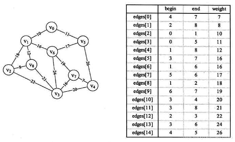
public void createEdgeArray() {
Edge edge0 = new Edge(4, 7, 7);
Edge edge1 = new Edge(2, 8, 8);
Edge edge2 = new Edge(0, 1, 10);
Edge edge3 = new Edge(0, 5, 11);
Edge edge4 = new Edge(1, 8, 12);
Edge edge5 = new Edge(3, 7, 16);
Edge edge6 = new Edge(1, 6, 16);
Edge edge7 = new Edge(5, 6, 17);
Edge edge8 = new Edge(1, 2, 18);
Edge edge9 = new Edge(6, 7, 19);
Edge edge10 = new Edge(3, 4, 20);
Edge edge11 = new Edge(3, 8, 21);
Edge edge12 = new Edge(2, 3, 22);
Edge edge13 = new Edge(3, 6, 24);
Edge edge14 = new Edge(4, 5, 26);
edges[0] = edge0;
edges[1] = edge1;
edges[2] = edge2;
edges[3] = edge3;
edges[4] = edge4;
edges[5] = edge5;
edges[6] = edge6;
edges[7] = edge7;
edges[8] = edge8;
edges[9] = edge9;
edges[10] = edge10;
edges[11] = edge11;
edges[12] = edge12;
edges[13] = edge13;
edges[14] = edge14;
}
class Edge{
private int begin;
private int end;
private int weight;
public Edge(int begin, int end, int weight) {
this.begin = begin;
this.end = end;
this.weight = weight;
}
public int getBegin() {
return begin;
}
public void setBegin(int begin) {
this.begin = begin;
}
public int getEnd() {
return end;
}
public void setEnd(int end) {
this.end = end;
}
public int getWeight() {
return weight;
}
public void setWeight(int weight) {
this.weight = weight;
}
}
}
public void miniSpanTreeKruskal() {
	int m, n, sum = 0;
	int[] parent = new int[edgeSize];//以起点为下标,值为终点的数组
	for (int i = 0; i < edgeSize; i++) {
		parent[i] = 0;
	}
	for (int i = 0; i < edgeSize; i++) {
		n = find(parent,edges[i].begin);
		m = find(parent,edges[i].end);
		//保证不出现回环
		if(n != m) {
			parent[n] = m;
			System.out.println("起点:" + edges[i].begin + ",终点:"
					+ edges[i].end + ",权值:" + edges[i].weight);
			sum += edges[i].weight;
		}
	}
	System.out.println("sum = " + sum);
}

//查找数组,获取非回环的值,也就是说这里找到的是值为0的位置
private int find(int[] parent, int value) {
	while(parent[value] > 0) {
		value = parent[value];
	}
	return value;
}
测试
public static void main(String[] args) {
	GraphKruskal gKruskal = new GraphKruskal(15);
	gKruskal.createEdgeArray();
	gKruskal.miniSpanTreeKruskal();
}
输出结果
起点:4,终点:7,权值:7
起点:2,终点:8,权值:8
起点:0,终点:1,权值:10
起点:0,终点:5,权值:11
起点:1,终点:8,权值:12
起点:3,终点:7,权值:16
起点:1,终点:6,权值:16
起点:6,终点:7,权值:19
sum = 99
最短路径
最短路径在路径规划时候是经常使用到的
网转邻接矩阵
计算最短路径,采用迪杰斯特拉算法
#define MAXVEX 9
#define INFINITY 65535
typedef int Pathmatirx[MAXVEX]; //用于存储最短路径下标的数组
typedef int ShortPathTable[MAXVEX]; //用于存储到各点最短路径的权值和

//Dijkstra算法,求有向网G的v0顶点到其余顶点v最短路径P[v]及带权长度D[v]
//P[v]的值为前驱顶点下标,D[v]表示v0到v的最短路径长度和
void ShortestPath_Dijkstra(MGraph G,int v0,Pathmatrix *P,ShortPathTable *D){
	int v,w,k,min;
	int final[MAXVEX]; //final[w] = 1表示求得顶点v0至vw的最短路径
	for(v = 0; v < G.numVertexes; v++){ //初始化数据
		final[v] = 0; //全部顶点初始化为未知最短路径状态
		(*D)[v] = G.matirx[v0][v]; //将与v0点有连线的顶点加上权值
		(*P)[v] = 0; //初始化路径数组为0
	}
	(*D)[v0] = 0; //v0至v0的路径为0
	final[v0] = 1; //v0至v0不需要求路径
	//开始主循环,每次求得v0到某个v顶点的最短路径
	for(v = 1; v < G.numVertexes; v++){
		min = INFINITY; //当前所知离v0顶点的最近距离
		for(w = 0; w < G.numVertexes; w++){ //寻找离v0最近的顶点
			if(!final[w] && (*D)[w] < min){
				k = w;
				min = (*D)[w]; //w顶点离v0顶点更近
			}
		}
		final[k] = 1; //将目前找到的最近的顶点置为1
		for(w = 0; w < G.numVertexes; w++){ //修正当前最短路径与距离
			//如果经过v顶点的路径比现在这条路径的长度短的话
			if(!final[w] && (min + G.matirx[k][w] < (*D)[w])){
				//说明找到了更短的路径,修改D[w]和P[w]
				(*D)[w] = min + G.matirx[k][w]; //修改当前路径长度
				(*P)[w] = k;
			}
		}
	}
}
转化为Java
public class Dijkstra {
	private int MAXVEX;
	private int MAX_WEIGHT;
	private boolean isGetPath[];
	private int shortTablePath[];

	public void shortesPathDijkstra(Graph graph) {
		int min, k = 0;
		MAXVEX = graph.getVertexSize();
		MAX_WEIGHT = Graph.MAX_WEIGHT;
		shortTablePath = new int[MAXVEX];
		isGetPath = new boolean[MAXVEX];
		//初始化,拿到第一行位置
		for (int v = 0; v < graph.getVertexSize(); v++) {
			shortTablePath[v] = graph.getMatrix()[0][v];
		}
		//从V0开始,自身到自身的距离为0
		shortTablePath[0] = 0;
		isGetPath[0] = true;
		for (int v = 1; v < graph.getVertexSize(); v++) {
			min = MAX_WEIGHT;
			for (int w = 0; w < graph.getVertexSize(); w++) {
				//说明v和w有焦点
				if(!isGetPath[w] && shortTablePath[w] < min) {
					k = w;
					min = shortTablePath[w];
				}
			}
			isGetPath[k] = true;
			for (int u = 0; u < graph.getVertexSize(); u++) {
				if(!isGetPath[u] && (min + graph.getMatrix()[k][u]) < shortTablePath[u]) {
					shortTablePath[u] = min + graph.getMatrix()[k][u];
				}
			}
		}
		for (int i = 0; i < shortTablePath.length; i++) {
			System.out.println("V0到V" + i + "的最短路径为:" + shortTablePath[i]);
		}
	}

	public static void main(String[] args) {
		Graph graph = new Graph(9);
		graph.createGraph();
		Dijkstra dijkstra = new Dijkstra();
		dijkstra.shortesPathDijkstra(graph);
	}
}
测试数据
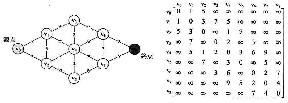
public class Graph {
	private int vertexSize; //顶点数量
	private int[] vertexs; //顶点数组
	private int[][] matrix; //边数组
	public static final int MAX_WEIGHT = 1000; //非连接顶点权值

	public Graph(int vertexSize) {
		this.vertexSize = vertexSize;
		this.vertexs = new int[vertexSize];
		this.matrix = new int[vertexSize][vertexSize];
		//顶点初始化
		for (int i = 0; i < vertexSize; i++) {
			vertexs[i]= i;
		}
	}

	public int getVertexSize() {
		return vertexSize;
	}

	public int[][] getMatrix() {
		return matrix;
	}

	public void createGraph(){
		int [] a1 = new int[]{0,1,5,MAX_WEIGHT,MAX_WEIGHT,MAX_WEIGHT,MAX_WEIGHT,MAX_WEIGHT,MAX_WEIGHT};
		int [] a2 = new int[]{1,0,3,7,5,MAX_WEIGHT,MAX_WEIGHT,MAX_WEIGHT,MAX_WEIGHT};
		int [] a3 = new int[]{5,3,0,MAX_WEIGHT,1,7,MAX_WEIGHT,MAX_WEIGHT,MAX_WEIGHT};
		int [] a4 = new int[]{MAX_WEIGHT,7,MAX_WEIGHT,0,2,MAX_WEIGHT,3,MAX_WEIGHT,MAX_WEIGHT};
		int [] a5 = new int[]{MAX_WEIGHT,5,1,2,0,3,6,9,MAX_WEIGHT};
		int [] a6 = new int[]{MAX_WEIGHT,MAX_WEIGHT,7,MAX_WEIGHT,3,0,MAX_WEIGHT,5,MAX_WEIGHT};
		int [] a7 = new int[]{MAX_WEIGHT,MAX_WEIGHT,MAX_WEIGHT,3,6,MAX_WEIGHT,0,2,7};
		int [] a8 = new int[]{MAX_WEIGHT,MAX_WEIGHT,MAX_WEIGHT,MAX_WEIGHT,9,5,2,0,4};
		int [] a9 = new int[]{MAX_WEIGHT,MAX_WEIGHT,MAX_WEIGHT,MAX_WEIGHT,MAX_WEIGHT,MAX_WEIGHT,7,4,0};

		matrix[0] = a1;
		matrix[1] = a2;
		matrix[2] = a3;
		matrix[3] = a4;
		matrix[4] = a5;
		matrix[5] = a6;
		matrix[6] = a7;
		matrix[7] = a8;
		matrix[8] = a9;
	}
}
拓扑排序
在一个表示工程的有向图中,用顶点表示活动,用弧表示活动之间的优先关系,这样的有向图为顶点表示活动的网,称之为AOV网(Activity On Vertex Network)
设G=(V,E)是一个具有n个顶点的有向图,V中的顶点序列v1,v2,···,vn满足若从顶点vi到vj有一条路径,则在顶点序列中顶点vi必在顶点vj之前,则我们称这样的顶点序列为一个拓扑序列
实现拓扑排序
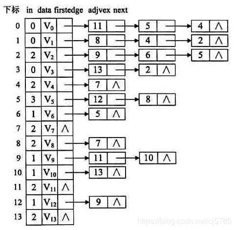
public class GraphTopologic {
private int numVertexes;
private VertexNode[] adjList;//邻接顶点的一维数组
public GraphTopologic(int numVertexes){
this.numVertexes = numVertexes;
}
//边表顶点
class EdgeNode{
private int adjVert; //下标
private EdgeNode next;
private int weight;
public EdgeNode(int adjVert) {
this.adjVert = adjVert;
}
}
//邻接顶点
class VertexNode{
private int in; //入度
private String data;
private EdgeNode firstEdge;
public VertexNode(int in, String data) {
this.in = in;
this.data = data;
}
}
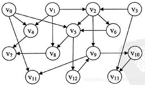
private void createGraph(){
VertexNode node0 = new VertexNode(0,"v0");
VertexNode node1 = new VertexNode(0,"v1");
VertexNode node2 = new VertexNode(2,"v2");
VertexNode node3 = new VertexNode(0,"v3");
VertexNode node4 = new VertexNode(2,"v4");
VertexNode node5 = new VertexNode(3,"v5");
VertexNode node6 = new VertexNode(1,"v6");
VertexNode node7 = new VertexNode(2,"v7");
VertexNode node8 = new VertexNode(2,"v8");
VertexNode node9 = new VertexNode(1,"v9");
VertexNode node10 = new VertexNode(1,"v10");
VertexNode node11 = new VertexNode(2,"v11");
VertexNode node12 = new VertexNode(1,"v12");
VertexNode node13 = new VertexNode(2,"v13");
adjList = new VertexNode[numVertexes];
adjList[0] =node0;
adjList[1] =node1;
adjList[2] =node2;
adjList[3] =node3;
adjList[4] =node4;
adjList[5] =node5;
adjList[6] =node6;
adjList[7] =node7;
adjList[8] =node8;
adjList[9] =node9;
adjList[10] =node10;
adjList[11] =node11;
adjList[12] =node12;
adjList[13] =node13;
node0.firstEdge = new EdgeNode(11);node0.firstEdge.next = new EdgeNode(5);node0.firstEdge.next.next = new EdgeNode(4);
node1.firstEdge = new EdgeNode(8);node1.firstEdge.next = new EdgeNode(4);node1.firstEdge.next.next = new EdgeNode(2);
node2.firstEdge = new EdgeNode(9);node2.firstEdge.next = new EdgeNode(6);node2.firstEdge.next.next = new EdgeNode(5);
node3.firstEdge = new EdgeNode(13);node3.firstEdge.next = new EdgeNode(2);
node4.firstEdge = new EdgeNode(7);
node5.firstEdge = new EdgeNode(12);node5.firstEdge.next = new EdgeNode(8);
node6.firstEdge = new EdgeNode(5);
node8.firstEdge = new EdgeNode(7);
node9.firstEdge = new EdgeNode(11);node9.firstEdge.next = new EdgeNode(10);
node10.firstEdge = new EdgeNode(13);
node12.firstEdge = new EdgeNode(9);
}
//拓扑排序
private void topologicalSort() throws Exception{
Stack<Integer> stack = new Stack<>();
int count = 0;
int k = 0;
for(int i = 0;i < numVertexes; i++){
if(adjList[i].in == 0){
stack.push(i);
}
}
while(!stack.isEmpty()){
int pop = stack.pop();
System.out.println("顶点:" + adjList[pop].data);
count++;
//遍历散列表中的链表
for(EdgeNode node = adjList[pop].firstEdge; node != null; node = node.next){
k = node.adjVert;//下标
if(--adjList[k].in == 0){
stack.push(k);//入度为0,入栈
}
}
}
if(count != numVertexes){
throw new Exception("拓扑排序失败");
}
}
public static void main(String[] args) {
GraphTopologic topologic = new GraphTopologic(14);
topologic.createGraph();
try {
topologic.topologicalSort();
} catch (Exception e) {
e.printStackTrace();
}
}
}
输出结果
顶点:v3
顶点:v1
顶点:v2
顶点:v6
顶点:v9
顶点:v10
顶点:v13
顶点:v0
顶点:v4
顶点:v5
顶点:v8
顶点:v7
顶点:v12
顶点:v11

 浙公网安备 33010602011771号