一个简单文本分类任务-EM算法-R语言

一、问题介绍

概率分布模型中，有时只含有可观测变量，如单硬币投掷模型，对于每个测试样例，硬币最终是正面还是反面是可以观测的。而有时还含有不可观测变量，如三硬币投掷模型。问题这样描述，首先投掷硬币A，如果是正面，则投掷硬币B，如果是反面，则投掷硬币C，最终只记录硬币B,C投掷的结果是正面还是反面，因此模型中硬币B,C的正反是可观测变量，而硬币A的正反则是不可观测变量。这里，用Y表示可观测变量，Z表示（隐变量）不可观测变量，Y和Z统称为完全数据，Y成为不完全数据。对于文本分类问题，未标记数据的自变量为可观测变量Y，未标记数据为观测到的类别标签为隐变量Z。
一般的只含有可观测变量的概率分布模型由于先验概率分布是可以通过可观测的类别标签来求得（对应文本分类问题中每个类别的数据出现的概率），而条件概率分布是可以通过可观测的类别标签以和可观测的样本自变量中特征来求得（对应文本分类问题中已知类别的前提下某个单词是否出现的概率），因此通过朴素贝叶斯法就可以对概率模型求解。但是如果模型中存在隐变量，那么朴素贝叶斯法则不能使用，因为先验概率分布和条件概率分布无法直接求得，因此提出一种用迭代方式进行的对不完全数据进行极大似然估计的方法——期望最大化算法（EM算法），接下来将对算法进行详细的证明和解释。

二、算法详解

1. 极大化似然函数

由于能观测到的数据只有不完全数据Y，因此对参数进行极大似然估计。

 

L（θ）=logP(Y∣θ)=log∑zP(Y,Z∣θ)=log∑zP(Y∣Z,θ)P(Z∣θ)

 

对Z前提下Y的概率分布可以理解为每个类别确定后Y的概率模型。如果是高斯混合模型，那么类别确定之后，自变量应该符合高斯分布，如果是文本分类模型，那么类别确定之后，自变量应该符合条件概率分布（自变量是特征的集合，由于所有特征都是条件独立的，因此联合分布就是各个特征的分布连乘在一起，每个特征满足两点分布，那么自变量应该满足连乘的两点分布）。对Z的先验概率分布可以理解为每个类别出现的比例，即每个类别的先验概率。不完全数据的Z是无法观测的，因此难点就在于确定条件概率分布和先验概率分布。

 

L(θ)≥B(θ，θ)=∑zP(Z∣Y,θ)logP(Y,Z∣θ)P(Z∣Y,θ)L(θ)≥B(θ，θ)=∑zP(Z∣Y,θ)log⁡P(Y,Z∣θ)P(Z∣Y,θ)

这里B的两个参数表示不同含义，前一个参数表示Z的后验概率分布的参数空间，后一个参数表示完全数据的联合分布。

 

2. 收敛性分析

现在最大化似然函数L，可以先求似然函数L的下限函数B，然后找出下限函数B的极大值点，那么该点一定也使似然函数L更靠近其极大值点，通过迭代的步骤，就可以不断逼近L的极值点。如下图EM算法迭代
首先用先验启动知识对Z的后验概率进行初始化，即用已标记数据及计算出Y前提下Z的概率分布，因此可获得P(Z∣Y,θ(0))P(Z∣Y,θ(0))，这样在初始点（自变量是参数空间，应变量是似然函数值）的下限函数就可以求出，当迭代到第t步时求出下限函数为B(θ(t),θ)B(θ(t),θ)在t这一点，似然函数L和其下限函数相等L（θ(t)）=B(θ(t),θ(t))L（θ(t)）=B(θ(t),θ(t))。这时对B求极大值，可以获得迭代的下一步的参数  

3. 算法流程

EM算法的流程分为两步，分别是E（期望）步和M（最大化）步。E步主要是求出当前的下限函数B，由于B是通过期望推导出的，所以称为期望步骤，M步主要是求出当前下限函数B的极大值，然后将这点的参数带入似然函数，所以称为最大化步，因此算法流程如下：
1. 利用预先知识，求出隐变量的后验概率分布，获得参数空间的初始值θ(0)来启动EM算法。
2. E步，求期望Ez[logP(Z,Y∣θ)∣Y,θ(t)]Ez[log⁡P(Z,Y∣θ)∣Y,θ(t)]
3. M步，最大化期望，求出新的参数值θ(t+1)θ(t+1)
4. 迭代2、3步直至收敛或固定的迭代次数

 

下面是数学推导部分

 

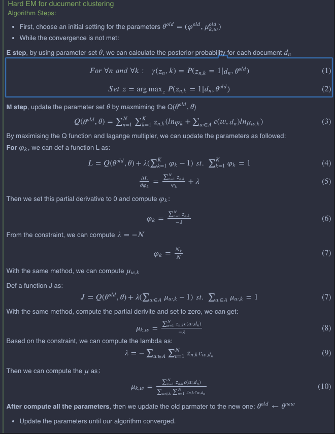
那根据上面的算法过程，我们可以讲其实现，代码如下

## Help Function
logSum <- function(v) {
   m = max(v)
   return ( m + log(sum(exp(v-m))))
}

# Hard E step
hard.E.step <- function(gamma, model, counts){
  # Model Parameter Setting
  N <- dim(counts)[2] # number of documents
  K <- dim(model$mu)[1]

  # E step:    
  for (n in 1:N){
    for (k in 1:K){
      ## calculate the posterior based on the estimated mu and rho in the "log space"
      gamma[n,k] <- log(model$rho[k,1]) +  sum(counts[,n] * log(model$mu[k,])) 
    }
    # normalisation to sum to 1 in the log space
    logZ = logSum(gamma[n,])
    gamma[n,] = gamma[n,] - logZ
  
    ## Compared with soft EM, here we need to do a hard assignment for the ducuments based on the post probability
    ## Find the max post probablity for znk
    max.index <- which.max(gamma[n,])
    ## Set all the post probability to 0 and biggest to 1 and finish the hard assignment
    gamma[n,] <- 0
    gamma[n,max.index] <- 1 
  }

  return (gamma)
}

　　

# M step
M.step <- function(gamma, model, counts,eps=1e-10){
  # Model Parameter Setting
    N <- dim(counts)[2]   # number of documents
    W <- dim(counts)[1]   # number of words i.e. vocabulary size
    K <- dim(model$mu)[1] # number of clusters

      ## Updating the parameters in the M step
    for (k in 1:K) {
        ## Update the mix cofficients 
        model$rho[k,1] <- sum(gamma[,k])/N
        ## Update the language model mu 
        total <- sum(gamma[,k] * t(counts)) + W * eps
        ## For each w, compute the language model
        for (w in 1:W){
            model$mu[k,w] <- (sum(gamma[,k] * counts[w,]) + eps)/total
        }  
        
    }
  
      # Return the result
      return (model)
}

　　

##--- Initialize model parameters randomly --------------------------------------------
##
initial.param <- function(vocab_size, K=4, seed=123456){
  rho <- matrix(1/K,nrow = K, ncol=1)                    # assume all clusters have the same size (we will update this later on)
  mu <- matrix(runif(K*vocab_size),nrow = K, ncol = vocab_size)    # initiate Mu 
  mu <- prop.table(mu, margin = 1)               # normalization to ensure that sum of each row is 1
  return (list("rho" = rho, "mu"= mu))
}

　接着我们把E-Mstep合并在一起

## Hard EM
##--- EM for Document Clustering --------------------------------------------
hard.EM <- function(counts, K=4, max.epoch=10, seed=123456){
  #INPUTS:
  ## counts: word count matrix
  ## K: the number of clusters
  #OUTPUTS:
  ## model: a list of model parameters
  
  # Model Parameter Setting
  N <- dim(counts)[2] # number of documents
  W <- dim(counts)[1] # number of unique words (in all documents)
  
  # Initialization
  model <- initial.param(W, K=K, seed=seed)
  gamma <- matrix(0, nrow = N, ncol = K)

  print(train_obj(model,counts))
  # Build the model
  for(epoch in 1:max.epoch){
    
    # E Step
    gamma <- hard.E.step(gamma, model, counts)
    # M Step
    model <- M.step(gamma, model, counts)
   
    print(train_obj(model,counts)) 
  }
  # Return Model
  return(list("model"=model,"gamma"=gamma))
}

　　

接着，我们需要导入我们的文本，并做简单处理，接着我们去验证下我们上面实现的EM代码

## Load the library
library(tm)
library(SnowballC)

## Function for reading the data
eps=1e-10
  
# reading the data
read.data <- function(file.name='Task2A.txt', sample.size=1000, seed=100, pre.proc=TRUE, spr.ratio= 0.90) {
  # INPUTS:
  ## file.name: name of the input .txt file
  ## sample.size: if == 0  reads all docs, otherwise only reads a subset of the corpus
  ## seed: random seed for sampling (read above)
  ## pre.proc: if TRUE performs the preprocessing (recommended)
  ## spr.ratio: is used to reduce the sparcity of data by removing very infrequent words
  # OUTPUTS:
  ## docs: the unlabled corpus (each row is a document)
  ## word.doc.mat: the count matrix (each rows and columns corresponds to words and documents, respectively)
  ## label: the real cluster labels (will be used in visualization/validation and not for clustering)
  
  # Read the data
  text <- readLines(file.name)
  # select a subset of data if sample.size > 0
  if (sample.size>0){
    set.seed(seed)
    text <- text[sample(length(text), sample.size)]
  }
  ## the terms before the first '\t' are the lables (the newsgroup names) and all the remaining text after '\t' are the actual documents
  docs <- strsplit(text, '\t')
  # store the labels for evaluation
  labels <-  unlist(lapply(docs, function(x) x[1]))
  # store the unlabeled texts    
  docs <- data.frame(unlist(lapply(docs, function(x) x[2])))
  
  
  library(tm)
  # create a corpus
  docs <- DataframeSource(docs)
  corp <- Corpus(docs)
  
  # Preprocessing:
  if (pre.proc){
    corp <- tm_map(corp, removeWords, stopwords("english")) # remove stop words (the most common word in a language that can be find in any document)
    corp <- tm_map(corp, removePunctuation) # remove pnctuation
    corp <- tm_map(corp, stemDocument) # perform stemming (reducing inflected and derived words to their root form)
    corp <- tm_map(corp, removeNumbers) # remove all numbers
    corp <- tm_map(corp, stripWhitespace) # remove redundant spaces 
  }  
  # Create a matrix which its rows are the documents and colomns are the words. 
  dtm <- DocumentTermMatrix(corp)
  ## reduce the sparcity of out dtm
  dtm <- removeSparseTerms(dtm, spr.ratio)
  ## convert dtm to a matrix
  word.doc.mat <- t(as.matrix(dtm))
  
  # Return the result
  return (list("docs" = docs, "word.doc.mat"= word.doc.mat, "labels" = labels))
}

　　训练模型

# Reading documents 
## Note: sample.size=0 means all read all documents!
##(for develiopment and debugging use a smaller subset e.g., sample.size = 40)
data <- read.data(file.name='Task2A.txt', sample.size=0, seed=100, pre.proc=TRUE, spr.ratio= .99)

# word-document frequency matrix 
counts <- data$word.doc.mat   

# calling the hard EM algorithm on the data with K = 4
hard.res <- hard.EM(counts, K = 4, max.epoch = 50)

    

　　得到以下输出

2171715
[1] 1952192
[1] 1942383
[1] 1938631
[1] 1937321
[1] 1936228
[1] 1935571
[1] 1935383
[1] 1935195
[1] 1935073
[1] 1935032
[1] 1934910
[1] 1934876
[1] 1934764
[1] 1934700
[1] 1934629
[1] 1934559
[1] 1934515
[1] 1934494
[1] 1934387
[1] 1934331
[1] 1934249
[1] 1934181
[1] 1934101
[1] 1933877
[1] 1933044
[1] 1929635
[1] 1927475
[1] 1926070
[1] 1925825
[1] 1925707
[1] 1925570
[1] 1925531
[1] 1925507
[1] 1925477
[1] 1925468
[1] 1925456
[1] 1925431
[1] 1925385
[1] 1925271
[1] 1925170
[1] 1925055
[1] 1924912
[1] 1924732
[1] 1924470
[1] 1924196
[1] 1923888
[1] 1923562
[1] 1923348
[1] 1923261
[1] 1923162

　　将我们的结果可视化出来

##--- Cluster Visualization -------------------------------------------------
cluster.viz <- function(doc.word.mat, color.vector, title=' '){
  p.comp <- prcomp(doc.word.mat, scale. = TRUE, center = TRUE)
  plot(p.comp$x, col=color.vector, pch=1,  main=title)
}


# hard EM clustering visualization
## find the culster with the maximum probability (since we have soft assignment here)
label.hat <- apply(hard.res$gamma, 1, which.max) 
## normalize the count matrix for better visualization
counts<-scale(counts) # only use when the dimensionality of the data (number of words) is large enough

## visualize the estimated clusters
cluster.viz(t(counts), label.hat, 'Estimated Clusters (Hard EM)')

 

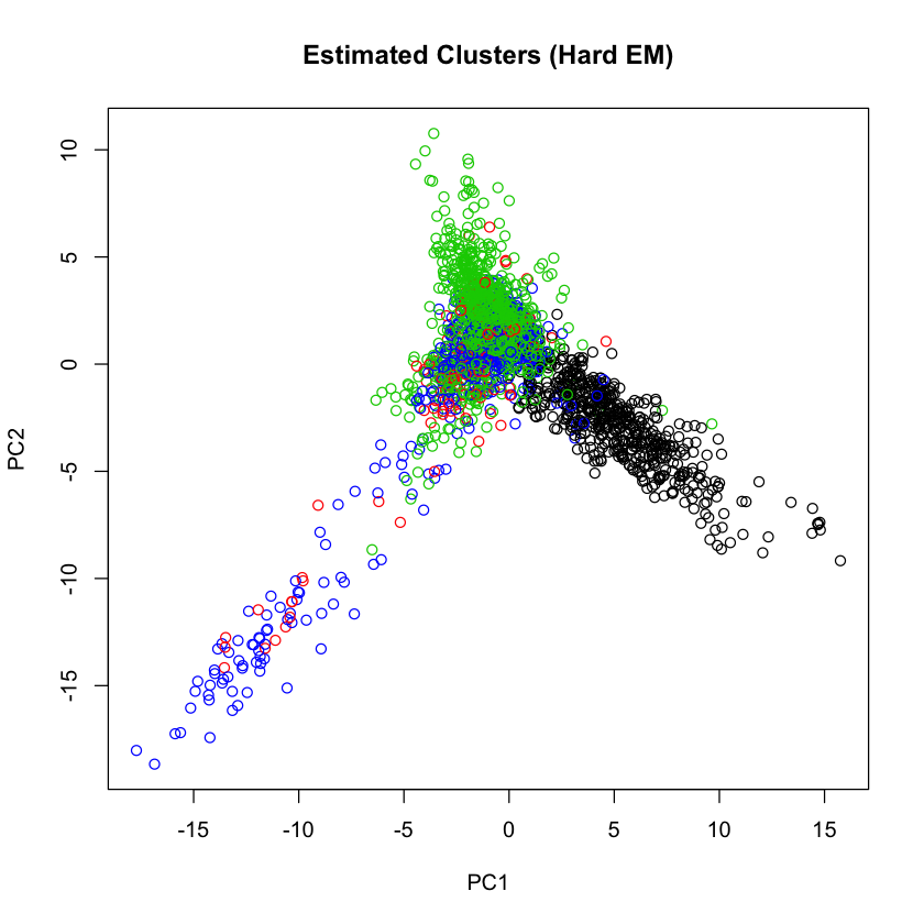
　　那这时候，我们把原文本直接分类可视化，和EM的分类做对比

## visualize the real clusters
cluster.viz(t(counts), factor(data$label), 'Real Clusters')

　　

　

 

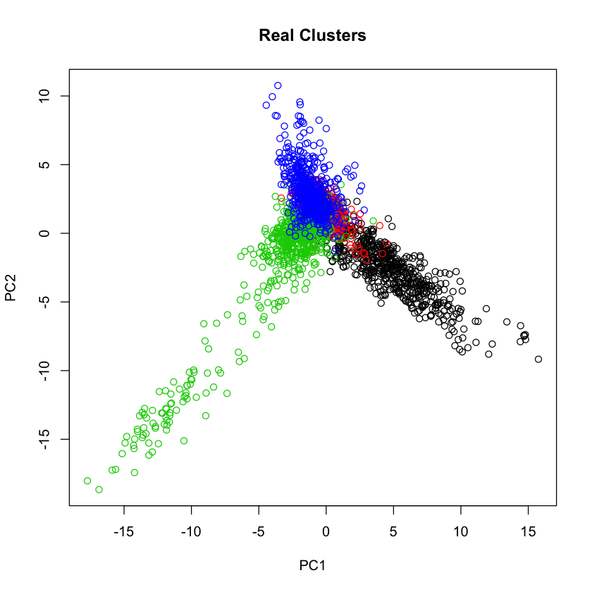
我们发现，EM基本上非常好的把文本的分类这个任务给完成了。