NLTK最详细功能介绍

一、前言

二、NLTK模块

三、使用 NLTK 分析单词和句子

四、NLTK 与停止词

五、NLTK 词干提取

六、NLTK 词性标注

七、NLTK 分块

八、 NLTK 添加缝隙（Chinking）

九、NLTK 命名实体识别

十、NLTK 词形还原

十一、NLTK 语料库

十二、 NLTK 和 Wordnet

十三、NLTK 文本分类

十四、使用 NLTK 将单词转换为特征

十五、NLTK 朴素贝叶斯分类器

十六、使用 NLTK 保存分类器

十七、NLTK 和 Sklearn

十八、使用 NLTK 组合算法

十九、使用 NLTK 调查偏差

二十、使用 NLTK 改善情感分析的训练数据

二十一、使用 NLTK 为情感分析创建模块

二十二、NLTK Twitter 情感分析

二十三，使用 NLTK 绘制 Twitter 实时情感分析

二十四、斯坦福 NER 标记器与命名实体识别

二十五、测试 NLTK 和斯坦福 NER 标记器的准确性

二十六、测试 NLTK 和斯坦福 NER 标记器的速度

二十七、使用 BIO 标签创建可读的命名实体列表

一、前言　

　　python进行自然语言处理，有一些第三方库供大家使用：

- NLTK（Python自然语言工具包）用于诸如标记化、词形还原、词干化、解析、POS标注等任务。该库具有几乎所有NLP任务的工具。
- Spacy是NLTK的主要竞争对手。这两个库可用于相同的任务。
- Scikit-learn为机器学习提供了一个大型库。此外还提供了用于文本预处理的工具。
- Gensim是一个主题和向量空间建模、文档集合相似性的工具包。
- Pattern库的一般任务是充当Web挖掘模块。因此，它仅支持自然语言处理（NLP）作为辅助任务。
- Polyglot是自然语言处理（NLP）的另一个Python工具包。它不是很受欢迎，但也可以用于各种NLP任务。

NLTK是一个高效的Python构建的平台，用来处理人类自然语言数据。它提供了易于使用的接口，通过这些接口可以访问超过50个语料库和词汇资源（如WordNet），还有一套用于分类、标记化、词干标记、解析和语义推理的文本处理库，以及工业级NLP库的封装器和一个活跃的讨论论坛。

二、NLTK模块

语言处理任务	NLTK模块	功能描述
获取和处理语料库	nltk.corpus	语料库和词典的标准化接口
字符串处理	nltk.tokenize, nltk.stem	分词，句子分解提取主干
搭配发现	nltk.collocations	t-检验，卡方，点互信息PMI
词性标识符	nltk.tag	n-gram, backoff, Brill, HMM, TnT
分类	nltk.classify, nltk.cluster	决策树，最大熵，贝叶斯，EM，k-means
分块	nltk.chunk	正则表达式，n-gram，命名实体
解析	nltk.parse	图表，基于特征，一致性，概率，依赖
语义解释	nltk.sem, nltk.inference	λ演算，一阶逻辑，模型检验
指标评测	nltk.metrics	精度，召回率，协议系数
概率与估计	nltk.probability	频率分布，平滑概率分布
应用	nltk.app nltk.chat	图形化的关键词排序，分析器，WordNet查看器，聊天机器人
语言学领域的工作	nltk.toolbox	处理SIL工具箱格式的数据

三、使用 NLTK 分析单词和句子

　　NLTK 模块是一个巨大的工具包，目的是在整个自然语言处理（NLP）方法上帮助您。 NLTK 将为您提供一切，从将段落拆分为句子，拆分词语，识别这些词语的词性，高亮主题，甚至帮助您的机器了解文本关于什么。在这个系列中，我们将要解决意见挖掘或情感分析的领域。

　　在我们学习如何使用 NLTK 进行情感分析的过程中，我们将学习以下内容：

- 分词 - 将文本正文分割为句子和单词。
- 词性标注
- 机器学习与朴素贝叶斯分类器
- 如何一起使用 Scikit Learn（sklearn）与 NLTK
- 用数据集训练分类器
- 用 Twitter 进行实时的流式情感分析。
- ...以及更多。

　　为了开始，你需要 NLTK 模块，以及 Python。

　　接下来，您需要 NLTK 3。安装 NLTK 模块的最简单方法是使用pip。

　　对于所有的用户来说，这通过打开cmd.exe，bash，或者你使用的任何 shell，并键入以下命令来完成：

pip install nltk

　　接下来，我们需要为 NLTK 安装一些组件。通过你的任何常用方式打开 python，然后键入：

import nltk
nltk.download()

　　除非你正在操作无头版本，否则一个 GUI 会弹出来，可能只有红色而不是绿色：

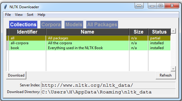
　　为所有软件包选择下载“全部”，然后单击“下载”。这会给你所有分词器，分块器，其他算法和所有的语料库。如果空间是个问题，您可以选择手动选择性下载所有内容。 NLTK 模块将占用大约 7MB，整个nltk_data目录将占用大约 1.8GB，其中包括您的分块器，解析器和语料库。

　　如果您正在使用 VPS 运行无头版本，您可以通过运行 Python ，并执行以下操作来安装所有内容：

import nltk

nltk.download()
d (for download)
all (for download everything)

　　这将为你下载一切东西。

　　现在你已经拥有了所有你需要的东西，让我们敲一些简单的词汇：

- 语料库（Corpus） - 文本的正文，单数。Corpora 是它的复数。示例：A collection of medical journals。
- 词库（Lexicon） - 词汇及其含义。例如：英文字典。但是，考虑到各个领域会有不同的词库。例如：对于金融投资者来说，Bull（牛市）这个词的第一个含义是对市场充满信心的人，与“普通英语词汇”相比，这个词的第一个含义是动物。因此，金融投资者，医生，儿童，机械师等都有一个特殊的词库。
- 标记（Token） - 每个“实体”都是根据规则分割的一部分。例如，当一个句子被“拆分”成单词时，每个单词都是一个标记。如果您将段落拆分为句子，则每个句子也可以是一个标记。

　　这些是在进入自然语言处理（NLP）领域时，最常听到的词语，但是我们将及时涵盖更多的词汇。以此，我们来展示一个例子，说明如何用 NLTK 模块将某些东西拆分为标记。

from nltk.tokenize import sent_tokenize, word_tokenize

EXAMPLE_TEXT = "Hello Mr. Smith, how are you doing today? The weather is great, and Python is awesome. The sky is pinkish-blue. You shouldn't eat cardboard."
print(sent_tokenize(EXAMPLE_TEXT))

　　起初，你可能会认为按照词或句子来分词，是一件相当微不足道的事情。对于很多句子来说，它可能是。第一步可能是执行一个简单的.split('. ')，或按照句号，然后是空格分割。之后也许你会引入一些正则表达式，来按照句号，空格，然后是大写字母分割。问题是像Mr. Smith这样的事情，还有很多其他的事情会给你带来麻烦。按照词分割也是一个挑战，特别是在考虑缩写的时候，例如we和we're。 NLTK 用这个看起来简单但非常复杂的操作为您节省大量的时间。

　　上面的代码会输出句子，分成一个句子列表，你可以用for循环来遍历。

['Hello Mr. Smith, how are you doing today?', 'The weather is great, and Python is awesome.', 'The sky is pinkish-blue.', "You shouldn't eat cardboard."]

　　所以这里，我们创建了标记，它们都是句子。让我们这次按照词来分词。

print(word_tokenize(EXAMPLE_TEXT))

['Hello', 'Mr.', 'Smith', ',', 'how', 'are', 'you', 'doing', 'today', '?', 'The', 'weather', 'is', 'great', ',', 'and', 'Python', 'is', 'awesome', '.', 'The', 'sky', 'is', 'pinkish-blue', '.', 'You', 'should', "n't", 'eat', 'cardboard', '.']

　　这里有几件事要注意。首先，注意标点符号被视为一个单独的标记。另外，注意单词shouldn't分隔为should和n't。最后要注意的是，pinkish-blue确实被当作“一个词”来对待，本来就是这样。很酷！

　　现在，看着这些分词后的单词，我们必须开始思考我们的下一步可能是什么。我们开始思考如何通过观察这些词汇来获得含义。我们可以想清楚，如何把价值放在许多单词上，但我们也看到一些基本上毫无价值的单词。这是一种“停止词”的形式，我们也可以处理。这就是我们将在下一个教程中讨论的内容。

四、NLTK 与停止词

　　自然语言处理的思想，是进行某种形式的分析或处理，机器至少可以在某种程度上理解文本的含义，表述或暗示。

　　这显然是一个巨大的挑战，但是有一些任何人都能遵循的步骤。然而，主要思想是电脑根本不会直接理解单词。令人震惊的是，人类也不会。在人类中，记忆被分解成大脑中的电信号，以发射模式的神经组的形式。对于大脑还有很多未知的事情，但是我们越是把人脑分解成基本的元素，我们就会发现基本的元素。那么，事实证明，计算机以非常相似的方式存储信息！如果我们要模仿人类如何阅读和理解文本，我们需要一种尽可能接近的方法。一般来说，计算机使用数字来表示一切事物，但是我们经常直接在编程中看到使用二进制信号（True或False，可以直接转换为 1 或 0，直接来源于电信号存在(True, 1)或不存在(False, 0)）。为此，我们需要一种方法,将单词转换为数值或信号模式。将数据转换成计算机可以理解的东西，这个过程称为“预处理”。预处理的主要形式之一就是过滤掉无用的数据。在自然语言处理中，无用词（数据）被称为停止词。

　　我们可以立即认识到，有些词语比其他词语更有意义。我们也可以看到，有些单词是无用的，是填充词。例如，我们在英语中使用它们来填充句子，这样就没有那么奇怪的声音了。一个最常见的，非官方的，无用词的例子是单词umm。人们经常用umm来填充，比别的词多一些。这个词毫无意义，除非我们正在寻找一个可能缺乏自信，困惑，或者说没有太多话的人。我们都这样做，有...呃...很多时候，你可以在视频中听到我说umm或uhh。对于大多数分析而言，这些词是无用的。

　　我们不希望这些词占用我们数据库的空间，或占用宝贵的处理时间。因此，我们称这些词为“无用词”，因为它们是无用的，我们希望对它们不做处理。 “停止词”这个词的另一个版本可以更书面一些：我们停在上面的单词。

　　例如，如果您发现通常用于讽刺的词语，可能希望立即停止。讽刺的单词或短语将因词库和语料库而异。就目前而言，我们将把停止词当作不含任何含义的词，我们要把它们删除。

　　您可以轻松地实现它，通过存储您认为是停止词的单词列表。 NLTK 用一堆他们认为是停止词的单词，来让你起步，你可以通过 NLTK 语料库来访问它：

from nltk.corpus import stopwords

　　这里是这个列表：

>>> set(stopwords.words('english'))
{'ourselves', 'hers', 'between', 'yourself', 'but', 'again', 'there', 'about', 'once', 'during', 'out', 'very', 'having', 'with', 'they', 'own', 'an', 'be', 'some', 'for', 'do', 'its', 'yours', 'such', 'into', 'of', 'most', 'itself', 'other', 'off', 'is', 's', 'am', 'or', 'who', 'as', 'from', 'him', 'each', 'the', 'themselves', 'until', 'below', 'are', 'we', 'these', 'your', 'his', 'through', 'don', 'nor', 'me', 'were', 'her', 'more', 'himself', 'this', 'down', 'should', 'our', 'their', 'while', 'above', 'both', 'up', 'to', 'ours', 'had', 'she', 'all', 'no', 'when', 'at', 'any', 'before', 'them', 'same', 'and', 'been', 'have', 'in', 'will', 'on', 'does', 'yourselves', 'then', 'that', 'because', 'what', 'over', 'why', 'so', 'can', 'did', 'not', 'now', 'under', 'he', 'you', 'herself', 'has', 'just', 'where', 'too', 'only', 'myself', 'which', 'those', 'i', 'after', 'few', 'whom', 't', 'being', 'if', 'theirs', 'my', 'against', 'a', 'by', 'doing', 'it', 'how', 'further', 'was', 'here', 'than'}

　　以下是结合使用stop_words集合，从文本中删除停止词的方法：

from nltk.corpus import stopwords
from nltk.tokenize import word_tokenize


example_sent = "This is a sample sentence, showing off the stop words filtration."

stop_words = set(stopwords.words('english'))

word_tokens = word_tokenize(example_sent)

filtered_sentence = [w for w in word_tokens if not w in stop_words]

filtered_sentence = []

for w in word_tokens:
    if w not in stop_words:
        filtered_sentence.append(w)

print(word_tokens)
print(filtered_sentence)

　　我们的输出是：

['This', 'is', 'a', 'sample', 'sentence', ',', 'showing', 'off', 'the', 'stop', 'words', 'filtration', '.']
['This', 'sample', 'sentence', ',', 'showing', 'stop', 'words', 'filtration', '.']

　　我们的数据库感谢了我们。数据预处理的另一种形式是“词干提取（Stemming）”，这就是我们接下来要讨论的内容。

五、NLTK 词干提取

　　词干的概念是一种规范化方法。除涉及时态之外，许多词语的变体都具有相同的含义。

　　我们提取词干的原因是为了缩短查找的时间，使句子正常化。

　　考虑：

I was taking a ride in the car.
I was riding in the car.

　　这两句话意味着同样的事情。 in the car（在车上）是一样的。 I（我）是一样的。在这两种情况下，ing都明确表示过去式，所以在试图弄清这个过去式活动的含义的情况下，是否真的有必要区分riding和taking a ride？

　　不，并没有。

　　这只是一个小例子，但想象英语中的每个单词，可以放在单词上的每个可能的时态和词缀。每个版本有单独的字典条目，将非常冗余和低效，特别是因为一旦我们转换为数字，“价值”将是相同的。

　　最流行的瓷感提取算法之一是 Porter，1979 年就存在了。

　　首先，我们要抓取并定义我们的词干：

from nltk.stem import PorterStemmer
from nltk.tokenize import sent_tokenize, word_tokenize

ps = PorterStemmer()

　　现在让我们选择一些带有相似词干的单词，例如：

example_words = ["python","pythoner","pythoning","pythoned","pythonly"]

　　下面，我们可以这样做来轻易提取词干：

for w in example_words:
    print(ps.stem(w))

　　我们的输出：

python
python
python
python
pythonli

　　现在让我们尝试对一个典型的句子，而不是一些单词提取词干：

new_text = "It is important to by very pythonly while you are pythoning with python. All pythoners have pythoned poorly at least once."
words = word_tokenize(new_text)

for w in words:
    print(ps.stem(w))

　　现在我们的结果为：

It
is
import
to
by
veri
pythonli
while
you
are
python
with
python
.
All
python
have
python
poorli
at
least
onc
.

　　接下来，我们将讨论 NLTK 模块中一些更高级的内容，词性标注，其中我们可以使用 NLTK 模块来识别句子中每个单词的词性。

六、NLTK 词性标注

　　NLTK模块的一个更强大的方面是，它可以为你做词性标注。意思是把一个句子中的单词标注为名词，形容词，动词等。更令人印象深刻的是，它也可以按照时态来标记，以及其他。这是一列标签，它们的含义和一些例子：

POS tag list:

CC  coordinating conjunction
CD  cardinal digit
DT  determiner
EX  existential there (like: "there is" ... think of it like "there exists")
FW  foreign word
IN  preposition/subordinating conjunction
JJ  adjective   'big'
JJR adjective, comparative  'bigger'
JJS adjective, superlative  'biggest'
LS  list marker 1)
MD  modal   could, will
NN  noun, singular 'desk'
NNS noun plural 'desks'
NNP proper noun, singular   'Harrison'
NNPS    proper noun, plural 'Americans'
PDT predeterminer   'all the kids'
POS possessive ending   parent's
PRP personal pronoun    I, he, she
PRP$    possessive pronoun  my, his, hers
RB  adverb  very, silently,
RBR adverb, comparative better
RBS adverb, superlative best
RP  particle    give up
TO  to  go 'to' the store.
UH  interjection    errrrrrrrm
VB  verb, base form take
VBD verb, past tense    took
VBG verb, gerund/present participle taking
VBN verb, past participle   taken
VBP verb, sing. present, non-3d take
VBZ verb, 3rd person sing. present  takes
WDT wh-determiner   which
WP  wh-pronoun  who, what
WP$ possessive wh-pronoun   whose
WRB wh-abverb   where, when

　　我们如何使用这个？当我们处理它的时候，我们要讲解一个新的句子标记器，叫做PunktSentenceTokenizer。这个标记器能够无监督地进行机器学习，所以你可以在你使用的任何文本上进行实际的训练。首先，让我们获取一些我们打算使用的导入：

import nltk
from nltk.corpus import state_union
from nltk.tokenize import PunktSentenceTokenizer

　　现在让我们创建训练和测试数据：

train_text = state_union.raw("2005-GWBush.txt")
sample_text = state_union.raw("2006-GWBush.txt")

　　一个是 2005 年以来的国情咨文演说，另一个是 2006 年以来的乔治·W·布什总统的演讲。

　　接下来，我们可以训练 Punkt 标记器，如下所示：

custom_sent_tokenizer = PunktSentenceTokenizer(train_text)

　　之后我们可以实际分词，使用：

tokenized = custom_sent_tokenizer.tokenize(sample_text)

　　现在我们可以通过创建一个函数，来完成这个词性标注脚本，该函数将遍历并标记每个句子的词性，如下所示：

def process_content():
    try:
        for i in tokenized[:5]:
            words = nltk.word_tokenize(i)
            tagged = nltk.pos_tag(words)
            print(tagged)

    except Exception as e:
        print(str(e))


process_content()

　　输出应该是元组列表，元组中的第一个元素是单词，第二个元素是词性标签。它应该看起来像：

[('PRESIDENT', 'NNP'), ('GEORGE', 'NNP'), ('W.', 'NNP'), ('BUSH', 'NNP'), ("'S", 'POS'), ('ADDRESS', 'NNP'), ('BEFORE', 'NNP'), ('A', 'NNP'), ('JOINT', 'NNP'), ('SESSION', 'NNP'), ('OF', 'NNP'), ('THE', 'NNP'), ('CONGRESS', 'NNP'), ('ON', 'NNP'), ('THE', 'NNP'), ('STATE', 'NNP'), ('OF', 'NNP'), ('THE', 'NNP'), ('UNION', 'NNP'), ('January', 'NNP'), ('31', 'CD'), (',', ','), ('2006', 'CD'), ('THE', 'DT'), ('PRESIDENT', 'NNP'), (':', ':'), ('Thank', 'NNP'), ('you', 'PRP'), ('all', 'DT'), ('.', '.')] [('Mr.', 'NNP'), ('Speaker', 'NNP'), (',', ','), ('Vice', 'NNP'), ('President', 'NNP'), ('Cheney', 'NNP'), (',', ','), ('members', 'NNS'), ('of', 'IN'), ('Congress', 'NNP'), (',', ','), ('members', 'NNS'), ('of', 'IN'), ('the', 'DT'), ('Supreme', 'NNP'), ('Court', 'NNP'), ('and', 'CC'), ('diplomatic', 'JJ'), ('corps', 'NNS'), (',', ','), ('distinguished', 'VBD'), ('guests', 'NNS'), (',', ','), ('and', 'CC'), ('fellow', 'JJ'), ('citizens', 'NNS'), (':', ':'), ('Today', 'NN'), ('our', 'PRP$'), ('nation', 'NN'), ('lost', 'VBD'), ('a', 'DT'), ('beloved', 'VBN'), (',', ','), ('graceful', 'JJ'), (',', ','), ('courageous', 'JJ'), ('woman', 'NN'), ('who', 'WP'), ('called', 'VBN'), ('America', 'NNP'), ('to', 'TO'), ('its', 'PRP$'), ('founding', 'NN'), ('ideals', 'NNS'), ('and', 'CC'), ('carried', 'VBD'), ('on', 'IN'), ('a', 'DT'), ('noble', 'JJ'), ('dream', 'NN'), ('.', '.')] [('Tonight', 'NNP'), ('we', 'PRP'), ('are', 'VBP'), ('comforted', 'VBN'), ('by', 'IN'), ('the', 'DT'), ('hope', 'NN'), ('of', 'IN'), ('a', 'DT'), ('glad', 'NN'), ('reunion', 'NN'), ('with', 'IN'), ('the', 'DT'), ('husband', 'NN'), ('who', 'WP'), ('was', 'VBD'), ('taken', 'VBN'), ('so', 'RB'), ('long', 'RB'), ('ago', 'RB'), (',', ','), ('and', 'CC'), ('we', 'PRP'), ('are', 'VBP'), ('grateful', 'JJ'), ('for', 'IN'), ('the', 'DT'), ('good', 'NN'), ('life', 'NN'), ('of', 'IN'), ('Coretta', 'NNP'), ('Scott', 'NNP'), ('King', 'NNP'), ('.', '.')] [('(', 'NN'), ('Applause', 'NNP'), ('.', '.'), (')', ':')] [('President', 'NNP'), ('George', 'NNP'), ('W.', 'NNP'), ('Bush', 'NNP'), ('reacts', 'VBZ'), ('to', 'TO'), ('applause', 'VB'), ('during', 'IN'), ('his', 'PRP$'), ('State', 'NNP'), ('of', 'IN'), ('the', 'DT'), ('Union', 'NNP'), ('Address', 'NNP'), ('at', 'IN'), ('the', 'DT'), ('Capitol', 'NNP'), (',', ','), ('Tuesday', 'NNP'), (',', ','), ('Jan', 'NNP'), ('.', '.')]

　　到了这里，我们可以开始获得含义，但是还有一些工作要做。我们将要讨论的下一个话题是分块（chunking），其中我们跟句单词的词性，将单词分到，有意义的分组中。

七、NLTK 分块

　　现在我们知道了词性，我们可以注意所谓的分块，把词汇分成有意义的块。分块的主要目标之一是将所谓的“名词短语”分组。这些是包含一个名词的一个或多个单词的短语，可能是一些描述性词语，也可能是一个动词，也可能是一个副词。这个想法是把名词和与它们有关的词组合在一起。

　　为了分块，我们将词性标签与正则表达式结合起来。主要从正则表达式中，我们要利用这些东西：

+ = match 1 or more
? = match 0 or 1 repetitions.
* = match 0 or MORE repetitions   
. = Any character except a new line

　　如果您需要正则表达式的帮助，请参阅上面链接的教程。最后需要注意的是，词性标签中用<和>表示，我们也可以在标签本身中放置正则表达式，来表达“全部名词”（<N.*>）。

import nltk
from nltk.corpus import state_union
from nltk.tokenize import PunktSentenceTokenizer

train_text = state_union.raw("2005-GWBush.txt")
sample_text = state_union.raw("2006-GWBush.txt")

custom_sent_tokenizer = PunktSentenceTokenizer(train_text)

tokenized = custom_sent_tokenizer.tokenize(sample_text)

def process_content():
    try:
        for i in tokenized:
            words = nltk.word_tokenize(i)
            tagged = nltk.pos_tag(words)
            chunkGram = r"""Chunk: {<RB.?>*<VB.?>*<NNP>+<NN>?}"""
            chunkParser = nltk.RegexpParser(chunkGram)
            chunked = chunkParser.parse(tagged)
            chunked.draw()     

    except Exception as e:
        print(str(e))

process_content()

　　结果是这样的：

　　这里的主要一行是：

chunkGram = r"""Chunk: {<RB.?>*<VB.?>*<NNP>+<NN>?}"""

　　把这一行拆分开：

　　<RB.?>*：零个或多个任何时态的副词，后面是：

　　<VB.?>*：零个或多个任何时态的动词，后面是：

　　<NNP>+：一个或多个合理的名词，后面是：

　　<NN>?：零个或一个名词单数。

　　尝试玩转组合来对各种实例进行分组，直到您觉得熟悉了。

　　视频中没有涉及，但是也有个合理的任务是实际访问具体的块。这是很少被提及的，但根据你在做的事情，这可能是一个重要的步骤。假设你把块打印出来，你会看到如下输出：

(S
  (Chunk PRESIDENT/NNP GEORGE/NNP W./NNP BUSH/NNP)
  'S/POS
  (Chunk
    ADDRESS/NNP
    BEFORE/NNP
    A/NNP
    JOINT/NNP
    SESSION/NNP
    OF/NNP
    THE/NNP
    CONGRESS/NNP
    ON/NNP
    THE/NNP
    STATE/NNP
    OF/NNP
    THE/NNP
    UNION/NNP
    January/NNP)
  31/CD
  ,/,
  2006/CD
  THE/DT
  (Chunk PRESIDENT/NNP)
  :/:
  (Chunk Thank/NNP)
  you/PRP
  all/DT
  ./.)

　　很酷，这可以帮助我们可视化，但如果我们想通过我们的程序访问这些数据呢？那么，这里发生的是我们的“分块”变量是一个 NLTK 树。每个“块”和“非块”是树的“子树”。我们可以通过像chunked.subtrees的东西来引用它们。然后我们可以像这样遍历这些子树：

 for subtree in chunked.subtrees():
     print(subtree)

　　接下来，我们可能只关心获得这些块，忽略其余部分。我们可以在chunked.subtrees()调用中使用filter参数。

for subtree in chunked.subtrees(filter=lambda t: t.label() == 'Chunk'):
    print(subtree)

　　现在，我们执行过滤，来显示标签为“块”的子树。请记住，这不是 NLTK 块属性中的“块”...这是字面上的“块”，因为这是我们给它的标签：chunkGram = r"""Chunk: {<RB.?>*<VB.?>*<NNP>+<NN>?}"""。

　　如果我们写了一些东西，类似chunkGram = r"""Pythons: {<RB.?>*<VB.?>*<NNP>+<NN>?}"""，那么我们可以通过"Pythons."标签来过滤。结果应该是这样的：

-
(Chunk PRESIDENT/NNP GEORGE/NNP W./NNP BUSH/NNP)
(Chunk
  ADDRESS/NNP
  BEFORE/NNP
  A/NNP
  JOINT/NNP
  SESSION/NNP
  OF/NNP
  THE/NNP
  CONGRESS/NNP
  ON/NNP
  THE/NNP
  STATE/NNP
  OF/NNP
  THE/NNP
  UNION/NNP
  January/NNP)
(Chunk PRESIDENT/NNP)
(Chunk Thank/NNP)

　　完整的代码是：

import nltk
from nltk.corpus import state_union
from nltk.tokenize import PunktSentenceTokenizer

train_text = state_union.raw("2005-GWBush.txt")
sample_text = state_union.raw("2006-GWBush.txt")

custom_sent_tokenizer = PunktSentenceTokenizer(train_text)

tokenized = custom_sent_tokenizer.tokenize(sample_text)

def process_content():
    try:
        for i in tokenized:
            words = nltk.word_tokenize(i)
            tagged = nltk.pos_tag(words)
            chunkGram = r"""Chunk: {<RB.?>*<VB.?>*<NNP>+<NN>?}"""
            chunkParser = nltk.RegexpParser(chunkGram)
            chunked = chunkParser.parse(tagged)
            
            print(chunked)
            for subtree in chunked.subtrees(filter=lambda t: t.label() == 'Chunk'):
                print(subtree)

            chunked.draw()

    except Exception as e:
        print(str(e))

process_content()

八、 NLTK 添加缝隙（Chinking）

　　你可能会发现，经过大量的分块之后，你的块中还有一些你不想要的单词，但是你不知道如何通过分块来摆脱它们。你可能会发现添加缝隙是你的解决方案。

　　添加缝隙与分块很像，它基本上是一种从块中删除块的方法。你从块中删除的块就是你的缝隙。

　　代码非常相似，你只需要用}{来代码缝隙，在块后面，而不是块的{}。

import nltk
from nltk.corpus import state_union
from nltk.tokenize import PunktSentenceTokenizer

train_text = state_union.raw("2005-GWBush.txt")
sample_text = state_union.raw("2006-GWBush.txt")

custom_sent_tokenizer = PunktSentenceTokenizer(train_text)

tokenized = custom_sent_tokenizer.tokenize(sample_text)

def process_content():
    try:
        for i in tokenized[5:]:
            words = nltk.word_tokenize(i)
            tagged = nltk.pos_tag(words)

            chunkGram = r"""Chunk: {<.*>+}
                                    }<VB.?|IN|DT|TO>+{"""

            chunkParser = nltk.RegexpParser(chunkGram)
            chunked = chunkParser.parse(tagged)

            chunked.draw()

    except Exception as e:
        print(str(e))

process_content()

　　使用它，你得到了一些东西：

　　现在，主要的区别是：

}<VB.?|IN|DT|TO>+{

　　这意味着我们要从缝隙中删除一个或多个动词，介词，限定词或to这个词。

　　现在我们已经学会了，如何执行一些自定义的分块和添加缝隙，我们来讨论一下 NLTK 自带的分块形式，这就是命名实体识别。

九、NLTK 命名实体识别

　　自然语言处理中最主要的分块形式之一被称为“命名实体识别”。这个想法是让机器立即能够拉出“实体”，例如人物，地点，事物，位置，货币等等。

　　这可能是一个挑战，但 NLTK 是为我们内置了它。 NLTK 的命名实体识别有两个主要选项：识别所有命名实体，或将命名实体识别为它们各自的类型，如人物，地点，位置等。

　　这是一个例子：

import nltk
from nltk.corpus import state_union
from nltk.tokenize import PunktSentenceTokenizer

train_text = state_union.raw("2005-GWBush.txt")
sample_text = state_union.raw("2006-GWBush.txt")

custom_sent_tokenizer = PunktSentenceTokenizer(train_text)

tokenized = custom_sent_tokenizer.tokenize(sample_text)

def process_content():
    try:
        for i in tokenized[5:]:
            words = nltk.word_tokenize(i)
            tagged = nltk.pos_tag(words)
            namedEnt = nltk.ne_chunk(tagged, binary=True)
            namedEnt.draw()
    except Exception as e:
        print(str(e))


process_content()

　　在这里，选择binary = True，这意味着一个东西要么是命名实体，要么不是。将不会有进一步的细节。结果是：

　　如果你设置了binary = False，结果为：

　　你可以马上看到一些事情。当binary是假的时候，它也选取了同样的东西，但是把White House这样的术语分解成White和House，就好像它们是不同的，而我们可以在binary = True的选项中看到，命名实体的识别说White House是相同命名实体的一部分，这是正确的。

　　根据你的目标，你可以使用binary选项。如果您的binary为false，这里是你可以得到的，命名实体的类型：

NE Type and Examples
ORGANIZATION - Georgia-Pacific Corp., WHO
PERSON - Eddy Bonte, President Obama
LOCATION - Murray River, Mount Everest
DATE - June, 2008-06-29
TIME - two fifty a m, 1:30 p.m.
MONEY - 175 million Canadian Dollars, GBP 10.40
PERCENT - twenty pct, 18.75 %
FACILITY - Washington Monument, Stonehenge
GPE - South East Asia, Midlothian

　　无论哪种方式，你可能会发现，你需要做更多的工作才能做到恰到好处，但是这个功能非常强大。

　　在接下来的教程中，我们将讨论类似于词干提取的东西，叫做“词形还原”（lemmatizing）。

十、NLTK 词形还原

　　与词干提权非常类似的操作称为词形还原。这两者之间的主要区别是，你之前看到了，词干提权经常可能创造出不存在的词汇，而词形是实际的词汇。

　　所以，你的词干，也就是你最终得到的词，不是你可以在字典中查找的东西，但你可以查找一个词形。

　　有时你最后会得到非常相似的词语，但有时候，你会得到完全不同的词语。我们来看一些例子。

from nltk.stem import WordNetLemmatizer

lemmatizer = WordNetLemmatizer()

print(lemmatizer.lemmatize("cats"))
print(lemmatizer.lemmatize("cacti"))
print(lemmatizer.lemmatize("geese"))
print(lemmatizer.lemmatize("rocks"))
print(lemmatizer.lemmatize("python"))
print(lemmatizer.lemmatize("better", pos="a"))
print(lemmatizer.lemmatize("best", pos="a"))
print(lemmatizer.lemmatize("run"))
print(lemmatizer.lemmatize("run",'v'))

　　在这里，我们有一些我们使用的词的词形的例子。唯一要注意的是，lemmatize接受词性参数pos。如果没有提供，默认是“名词”。这意味着，它将尝试找到最接近的名词，这可能会给你造成麻烦。如果你使用词形还原，请记住！

　　在接下来的教程中，我们将深入模块附带的 NTLK 语料库，查看所有优秀文档，他们在那里等待着我们。

十一、 NLTK 语料库

　　NLTK 语料库中的几乎所有文件都遵循相同的规则，通过使用 NLTK 模块来访问它们，但是它们没什么神奇的。这些文件大部分都是纯文本文件，其中一些是 XML 文件，另一些是其他格式文件，但都可以通过手动或模块和 Python 访问。让我们来谈谈手动查看它们。根据您的安装，您的nltk_data目录可能隐藏在多个位置。为了找出它的位置，请转到您的 Python 目录，也就是 NLTK 模块所在的位置。如果您不知道在哪里，请使用以下代码：

import nltk
print(nltk.__file__)

　　运行它，输出将是 NLTK 模块__init__.py的位置。进入 NLTK 目录，然后查找data.py文件。

　　代码的重要部分是：

if sys.platform.startswith('win'):
    # Common locations on Windows:
    path += [
        str(r'C:\nltk_data'), str(r'D:\nltk_data'), str(r'E:\nltk_data'),
        os.path.join(sys.prefix, str('nltk_data')),
        os.path.join(sys.prefix, str('lib'), str('nltk_data')),
        os.path.join(os.environ.get(str('APPDATA'), str('C:\\')), str('nltk_data'))
    ]
else:
    # Common locations on UNIX & OS X:
    path += [
        str('/usr/share/nltk_data'),
        str('/usr/local/share/nltk_data'),
        str('/usr/lib/nltk_data'),
        str('/usr/local/lib/nltk_data')
    ]

　　在那里，你可以看到nltk_data的各种可能的目录。如果你在 Windows 上，它很可能是在你的appdata中，在本地目录中。为此，你需要打开你的文件浏览器，到顶部，然后输入%appdata%。

　　接下来点击roaming，然后找到nltk_data目录。在那里，你将找到你的语料库文件。完整的路径是这样的：

C:\Users\yourname\AppData\Roaming\nltk_data\corpora

　　在这里，你有所有可用的语料库，包括书籍，聊天记录，电影评论等等。

　　现在，我们将讨论通过 NLTK 访问这些文档。正如你所看到的，这些主要是文本文档，所以你可以使用普通的 Python 代码来打开和阅读文档。也就是说，NLTK 模块有一些很好的处理语料库的方法，所以你可能会发现使用他们的方法是实用的。下面是我们打开“古腾堡圣经”，并阅读前几行的例子：

from nltk.tokenize import sent_tokenize, PunktSentenceTokenizer
from nltk.corpus import gutenberg

# sample text
sample = gutenberg.raw("bible-kjv.txt")

tok = sent_tokenize(sample)

for x in range(5):
    print(tok[x])

　　其中一个更高级的数据集是wordnet。 Wordnet 是一个单词，定义，他们使用的例子，同义词，反义词，等等的集合。接下来我们将深入使用 wordnet。

十二、NLTK 和 Wordnet

　　WordNet 是英语的词汇数据库，由普林斯顿创建，是 NLTK 语料库的一部分。

　　您可以一起使用 WordNet 和 NLTK 模块来查找单词含义，同义词，反义词等。我们来介绍一些例子。

　　首先，你将需要导入wordnet：

from nltk.corpus import wordnet

　　之后我们打算使用单词program来寻找同义词：

syns = wordnet.synsets("program")

　　一个同义词的例子：

print(syns[0].name())

# plan.n.01

　　只是单词：

print(syns[0].lemmas()[0].name())

# plan

　　第一个同义词的定义：

print(syns[0].definition())

# a series of steps to be carried out or goals to be accomplished

　　单词的使用示例：

print(syns[0].examples())

# ['they drew up a six-step plan', 'they discussed plans for a new bond issue']

　　接下来，我们如何辨别一个词的同义词和反义词？这些词形是同义词，然后你可以使用.antonyms找到词形的反义词。因此，我们可以填充一些列表，如：

synonyms = []
antonyms = []

for syn in wordnet.synsets("good"):
    for l in syn.lemmas():
        synonyms.append(l.name())
        if l.antonyms():
            antonyms.append(l.antonyms()[0].name())

print(set(synonyms))
print(set(antonyms))

'''
{'beneficial', 'just', 'upright', 'thoroughly', 'in_force', 'well', 'skilful', 'skillful', 'sound', 'unspoiled', 'expert', 'proficient', 'in_effect', 'honorable', 'adept', 'secure', 'commodity', 'estimable', 'soundly', 'right', 'respectable', 'good', 'serious', 'ripe', 'salutary', 'dear', 'practiced', 'goodness', 'safe', 'effective', 'unspoilt', 'dependable', 'undecomposed', 'honest', 'full', 'near', 'trade_good'} {'evil', 'evilness', 'bad', 'badness', 'ill'}
'''

　　你可以看到，我们的同义词比反义词更多，因为我们只是查找了第一个词形的反义词，但是你可以很容易地平衡这个，通过也为bad这个词执行完全相同的过程。

　　接下来，我们还可以很容易地使用 WordNet 来比较两个词的相似性和他们的时态，把 Wu 和 Palmer 方法结合起来用于语义相关性。

　　我们来比较名词ship和boat：

w1 = wordnet.synset('ship.n.01')
w2 = wordnet.synset('boat.n.01')
print(w1.wup_similarity(w2))

# 0.9090909090909091

w1 = wordnet.synset('ship.n.01')
w2 = wordnet.synset('car.n.01')
print(w1.wup_similarity(w2))

# 0.6956521739130435

w1 = wordnet.synset('ship.n.01')
w2 = wordnet.synset('cat.n.01')
print(w1.wup_similarity(w2))

# 0.38095238095238093

　　接下来，我们将讨论一些问题并开始讨论文本分类的主题。

十三、NLTK 文本分类

　　现在我们熟悉 NLTK 了，我们来尝试处理文本分类。文本分类的目标可能相当宽泛。也许我们试图将文本分类为政治或军事。也许我们试图按照作者的性别来分类。一个相当受欢迎的文本分类任务是，将文本的正文识别为垃圾邮件或非垃圾邮件，例如电子邮件过滤器。在我们的例子中，我们将尝试创建一个情感分析算法。

　　为此，我们首先尝试使用属于 NLTK 语料库的电影评论数据库。从那里，我们将尝试使用词汇作为“特征”，这是“正面”或“负面”电影评论的一部分。 NLTK 语料库movie_reviews数据集拥有评论，他们被标记为正面或负面。这意味着我们可以训练和测试这些数据。首先，让我们来预处理我们的数据。

import nltk
import random
from nltk.corpus import movie_reviews

documents = [(list(movie_reviews.words(fileid)), category)
             for category in movie_reviews.categories()
             for fileid in movie_reviews.fileids(category)]

random.shuffle(documents)

print(documents[1])

all_words = []
for w in movie_reviews.words():
    all_words.append(w.lower())

all_words = nltk.FreqDist(all_words)
print(all_words.most_common(15))
print(all_words["stupid"])

　　运行此脚本可能需要一些时间，因为电影评论数据集有点大。我们来介绍一下这里发生的事情。

　　导入我们想要的数据集后，您会看到：

documents = [(list(movie_reviews.words(fileid)), category)
             for category in movie_reviews.categories()
             for fileid in movie_reviews.fileids(category)]

　　基本上，用简单的英文，上面的代码被翻译成：在每个类别（我们有正向和独享），选取所有的文件 ID（每个评论有自己的 ID），然后对文件 ID存储word_tokenized版本（单词列表），后面是一个大列表中的正面或负面标签。

　　接下来，我们用random来打乱我们的文件。这是因为我们将要进行训练和测试。如果我们把他们按序排列，我们可能会训练所有的负面评论，和一些正面评论，然后在所有正面评论上测试。我们不想这样，所以我们打乱了数据。

　　然后，为了你能看到你正在使用的数据，我们打印出documents[1]，这是一个大列表，其中第一个元素是一列单词，第二个元素是pos或neg标签。

　　接下来，我们要收集我们找到的所有单词，所以我们可以有一个巨大的典型单词列表。从这里，我们可以执行一个频率分布，然后找出最常见的单词。正如你所看到的，最受欢迎的“词语”其实就是标点符号，the，a等等，但是很快我们就会得到有效词汇。我们打算存储几千个最流行的单词，所以这不应该是一个问题。

print(all_words.most_common(15))

　　以上给出了15个最常用的单词。你也可以通过下面的步骤找出一个单词的出现次数：

print(all_words["stupid"])

　　接下来，我们开始将我们的单词，储存为正面或负面的电影评论的特征。

十四、使用 NLTK 将单词转换为特征

　　编撰正面评论和负面评论中的单词的特征列表，来看到正面或负面评论中特定类型单词的趋势。

　　最初，我们的代码：

import nltk
import random
from nltk.corpus import movie_reviews

documents = [(list(movie_reviews.words(fileid)), category)
             for category in movie_reviews.categories()
             for fileid in movie_reviews.fileids(category)]

random.shuffle(documents)

all_words = []

for w in movie_reviews.words():
    all_words.append(w.lower())

all_words = nltk.FreqDist(all_words)

word_features = list(all_words.keys())[:3000]

　　几乎和以前一样，只是现在有一个新的变量，word_features，它包含了前 3000 个最常用的单词。接下来，我们将建立一个简单的函数，在我们的正面和负面的文档中找到这些前 3000 个单词，将他们的存在标记为是或否：

def find_features(document):
    words = set(document)
    features = {}
    for w in word_features:
        features[w] = (w in words)

    return features

　　下面，我们可以打印出特征集：

print((find_features(movie_reviews.words('neg/cv000_29416.txt'))))

　　之后我们可以为我们所有的文档做这件事情，通过做下列事情，保存特征存在性布尔值，以及它们各自的正面或负面的类别：

featuresets = [(find_features(rev), category) for (rev, category) in documents]

　　真棒，现在我们有了特征和标签，接下来是什么？通常，下一步是继续并训练算法，然后对其进行测试。所以，让我们继续这样做，从下一个教程中的朴素贝叶斯分类器开始！

十五、NLTK 朴素贝叶斯分类器

　　现在是时候选择一个算法，将我们的数据分成训练和测试集，然后启动！我们首先要使用的算法是朴素贝叶斯分类器。这是一个非常受欢迎的文本分类算法，所以我们只能先试一试。然而，在我们可以训练和测试我们的算法之前，我们需要先把数据分解成训练集和测试集。

　　你可以训练和测试同一个数据集，但是这会给你带来一些严重的偏差问题，所以你不应该训练和测试完全相同的数据。为此，由于我们已经打乱了数据集，因此我们将首先将包含正面和负面评论的 1900 个乱序评论作为训练集。然后，我们可以在最后的 100 个上测试，看看我们有多准确。

　　这被称为监督机器学习，因为我们正在向机器展示数据，并告诉它“这个数据是正面的”，或者“这个数据是负面的”。然后，在完成训练之后，我们向机器展示一些新的数据，并根据我们之前教过计算机的内容询问计算机，计算机认为新数据的类别是什么。

　　我们可以用以下方式分割数据：

# set that we'll train our classifier with
training_set = featuresets[:1900]

# set that we'll test against.
testing_set = featuresets[1900:]

　　下面，我们可以定义并训练我们的分类器：

classifier = nltk.NaiveBayesClassifier.train(training_set)

　　首先，我们只是简单调用朴素贝叶斯分类器，然后在一行中使用.train()进行训练。

　　足够简单，现在它得到了训练。接下来，我们可以测试它：

print("Classifier accuracy percent:",(nltk.classify.accuracy(classifier, testing_set))*100)

　　砰，你得到了你的答案。如果你错过了，我们可以“测试”数据的原因是，我们仍然有正确的答案。因此，在测试中，我们向计算机展示数据，而不提供正确的答案。如果它正确猜测我们所知的答案，那么计算机是正确的。考虑到我们所做的打乱，你和我可能准确度不同，但你应该看到准确度平均为 60-75%。

　　接下来，我们可以进一步了解正面或负面评论中最有价值的词汇：

classifier.show_most_informative_features(15)

　　这对于每个人都不一样，但是你应该看到这样的东西：

Most Informative Features
insulting = True neg : pos = 10.6 : 1.0
ludicrous = True neg : pos = 10.1 : 1.0
winslet = True pos : neg = 9.0 : 1.0
detract = True pos : neg = 8.4 : 1.0
breathtaking = True pos : neg = 8.1 : 1.0
silverstone = True neg : pos = 7.6 : 1.0
excruciatingly = True neg : pos = 7.6 : 1.0
warns = True pos : neg = 7.0 : 1.0
tracy = True pos : neg = 7.0 : 1.0
insipid = True neg : pos = 7.0 : 1.0
freddie = True neg : pos = 7.0 : 1.0
damon = True pos : neg = 5.9 : 1.0
debate = True pos : neg = 5.9 : 1.0
ordered = True pos : neg = 5.8 : 1.0
lang = True pos : neg = 5.7 : 1.0

　　这个告诉你的是，每一个词的负面到正面的出现几率，或相反。因此，在这里，我们可以看到，负面评论中的insulting一词比正面评论多出现 10.6 倍。Ludicrous是 10.1。

　　现在，让我们假设，你完全满意你的结果，你想要继续，也许使用这个分类器来预测现在的事情。训练分类器，并且每当你需要使用分类器时，都要重新训练，是非常不切实际的。因此，您可以使用pickle模块保存分类器。我们接下来做。

十六、使用 NLTK 保存分类器

　　训练分类器和机器学习算法可能需要很长时间，特别是如果您在更大的数据集上训练。我们的其实很小。你可以想象，每次你想开始使用分类器的时候，都要训练分类器吗？这么恐怖！相反，我们可以使用pickle模块，并序列化我们的分类器对象，这样我们所需要做的就是简单加载该文件。

　　那么，我们该怎么做呢？第一步是保存对象。为此，首先需要在脚本的顶部导入pickle，然后在使用.train()分类器进行训练后，可以调用以下几行：

save_classifier = open("naivebayes.pickle","wb")
pickle.dump(classifier, save_classifier)
save_classifier.close()

　　这打开了一个pickle文件，准备按字节写入一些数据。然后，我们使用pickle.dump()来转储数据。 pickle.dump()的第一个参数是你写入的东西，第二个参数是你写入它的地方。

　　之后，我们按照我们的要求关闭文件，这就是说，我们现在在脚本的目录中保存了一个pickle或序列化的对象！

　　接下来，我们如何开始使用这个分类器？ .pickle文件是序列化的对象，我们现在需要做的就是将其读入内存，这与读取任何其他普通文件一样简单。这样做：

classifier_f = open("naivebayes.pickle", "rb")
classifier = pickle.load(classifier_f)
classifier_f.close()

　　在这里，我们执行了非常相似的过程。我们打开文件来读取字节。然后，我们使用pickle.load()来加载文件，并将数据保存到分类器变量中。然后我们关闭文件，就是这样。我们现在有了和以前一样的分类器对象！

　　现在，我们可以使用这个对象，每当我们想用它来分类时，我们不再需要训练我们的分类器。

　　虽然这一切都很好，但是我们可能不太满意我们所获得的 60-75% 的准确度。其他分类器呢？其实，有很多分类器，但我们需要 scikit-learn（sklearn）模块。幸运的是，NLTK 的员工认识到将 sklearn 模块纳入 NLTK 的价值，他们为我们构建了一个小 API。这就是我们将在下一个教程中做的事情。

十七、NLTK 和 Sklearn

　　现在我们已经看到，使用分类器是多么容易，现在我们想尝试更多东西！ Python 的最好的模块是 Scikit-learn（sklearn）模块。

　　如果您想了解 Scikit-learn 模块的更多信息，我有一些关于 Scikit-Learn 机器学习的教程。

　　幸运的是，对于我们来说，NLTK 背后的人们更看重将 sklearn 模块纳入NLTK分类器方法的价值。就这样，他们创建了各种SklearnClassifier API。要使用它，你只需要像下面这样导入它：

from nltk.classify.scikitlearn import SklearnClassifier

　　从这里开始，你可以使用任何sklearn分类器。例如，让我们引入更多的朴素贝叶斯算法的变体：

from sklearn.naive_bayes import MultinomialNB,BernoulliNB

　　之后，如何使用它们？结果是，这非常简单。

MNB_classifier = SklearnClassifier(MultinomialNB())
MNB_classifier.train(training_set)
print("MultinomialNB accuracy percent:",nltk.classify.accuracy(MNB_classifier, testing_set))

BNB_classifier = SklearnClassifier(BernoulliNB())
BNB_classifier.train(training_set)
print("BernoulliNB accuracy percent:",nltk.classify.accuracy(BNB_classifier, testing_set))

　　就是这么简单。让我们引入更多东西：

from sklearn.linear_model import LogisticRegression,SGDClassifier
from sklearn.svm import SVC, LinearSVC, NuSVC

　　现在，我们所有分类器应该是这样：

print("Original Naive Bayes Algo accuracy percent:", (nltk.classify.accuracy(classifier, testing_set))*100)
classifier.show_most_informative_features(15)

MNB_classifier = SklearnClassifier(MultinomialNB())
MNB_classifier.train(training_set)
print("MNB_classifier accuracy percent:", (nltk.classify.accuracy(MNB_classifier, testing_set))*100)

BernoulliNB_classifier = SklearnClassifier(BernoulliNB())
BernoulliNB_classifier.train(training_set)
print("BernoulliNB_classifier accuracy percent:", (nltk.classify.accuracy(BernoulliNB_classifier, testing_set))*100)

LogisticRegression_classifier = SklearnClassifier(LogisticRegression())
LogisticRegression_classifier.train(training_set)
print("LogisticRegression_classifier accuracy percent:", (nltk.classify.accuracy(LogisticRegression_classifier, testing_set))*100)

SGDClassifier_classifier = SklearnClassifier(SGDClassifier())
SGDClassifier_classifier.train(training_set)
print("SGDClassifier_classifier accuracy percent:", (nltk.classify.accuracy(SGDClassifier_classifier, testing_set))*100)

SVC_classifier = SklearnClassifier(SVC())
SVC_classifier.train(training_set)
print("SVC_classifier accuracy percent:", (nltk.classify.accuracy(SVC_classifier, testing_set))*100)

LinearSVC_classifier = SklearnClassifier(LinearSVC())
LinearSVC_classifier.train(training_set)
print("LinearSVC_classifier accuracy percent:", (nltk.classify.accuracy(LinearSVC_classifier, testing_set))*100)

NuSVC_classifier = SklearnClassifier(NuSVC())
NuSVC_classifier.train(training_set)
print("NuSVC_classifier accuracy percent:", (nltk.classify.accuracy(NuSVC_classifier, testing_set))*100)

　　运行它的结果应该是这样：

Original Naive Bayes Algo accuracy percent: 63.0
Most Informative Features
                thematic = True              pos : neg    =      9.1 : 1.0
                secondly = True              pos : neg    =      8.5 : 1.0
                narrates = True              pos : neg    =      7.8 : 1.0
                 rounded = True              pos : neg    =      7.1 : 1.0
                 supreme = True              pos : neg    =      7.1 : 1.0
                 layered = True              pos : neg    =      7.1 : 1.0
                  crappy = True              neg : pos    =      6.9 : 1.0
               uplifting = True              pos : neg    =      6.2 : 1.0
                     ugh = True              neg : pos    =      5.3 : 1.0
                   mamet = True              pos : neg    =      5.1 : 1.0
                 gaining = True              pos : neg    =      5.1 : 1.0
                   wanda = True              neg : pos    =      4.9 : 1.0
                   onset = True              neg : pos    =      4.9 : 1.0
               fantastic = True              pos : neg    =      4.5 : 1.0
                kentucky = True              pos : neg    =      4.4 : 1.0
MNB_classifier accuracy percent: 66.0
BernoulliNB_classifier accuracy percent: 72.0
LogisticRegression_classifier accuracy percent: 64.0
SGDClassifier_classifier accuracy percent: 61.0
SVC_classifier accuracy percent: 45.0
LinearSVC_classifier accuracy percent: 68.0
NuSVC_classifier accuracy percent: 59.0

　　所以，我们可以看到，SVC 的错误比正确更常见，所以我们可能应该丢弃它。但是呢？接下来我们可以尝试一次使用所有这些算法。一个算法的算法！为此，我们可以创建另一个分类器，并根据其他算法的结果来生成分类器的结果。有点像投票系统，所以我们只需要奇数数量的算法。这就是我们将在下一个教程中讨论的内容。

十八、使用 NLTK 组合算法

　　现在我们知道如何使用一堆算法分类器，就像糖果岛上的一个孩子，告诉他们只能选择一个，我们可能会发现很难只选择一个分类器。好消息是，你不必这样！组合分类器算法是一种常用的技术，通过创建一种投票系统来实现，每个算法拥有一票，选择得票最多分类。

　　为此，我们希望我们的新分类器的工作方式像典型的 NLTK 分类器，并拥有所有方法。很简单，使用面向对象编程，我们可以确保从 NLTK 分类器类继承。为此，我们将导入它：

from nltk.classify import ClassifierI
from statistics import mode

　　我们也导入mode（众数），因为这将是我们选择最大计数的方法。

　　现在，我们来建立我们的分类器类：

class VoteClassifier(ClassifierI):
    def __init__(self, *classifiers):
        self._classifiers = classifiers

　　我们把我们的类叫做VoteClassifier，我们继承了 NLTK 的ClassifierI。接下来，我们将传递给我们的类的分类器列表赋给self._classifiers。

　　接下来，我们要继续创建我们自己的分类方法。我们打算把它称为.classify，以便我们可以稍后调用.classify，就像传统的 NLTK 分类器那样。

def classify(self, features):
        votes = []
        for c in self._classifiers:
            v = c.classify(features)
            votes.append(v)
        return mode(votes)

　　很简单，我们在这里所做的就是，遍历我们的分类器对象列表。然后，对于每一个，我们要求它基于特征分类。分类被视为投票。遍历完成后，我们返回mode(votes)，这只是返回投票的众数。

　　这是我们真正需要的，但是我认为另一个参数，置信度是有用的。由于我们有了投票算法，所以我们也可以统计支持和反对票数，并称之为“置信度”。例如，3/5 票的置信度弱于 5/5 票。因此，我们可以从字面上返回投票比例，作为一种置信度指标。这是我们的置信度方法：

 def confidence(self, features):
        votes = []
        for c in self._classifiers:
            v = c.classify(features)
            votes.append(v)

        choice_votes = votes.count(mode(votes))
        conf = choice_votes / len(votes)
        return conf

　　现在，让我们把东西放到一起：

import nltk
import random
from nltk.corpus import movie_reviews
from nltk.classify.scikitlearn import SklearnClassifier
import pickle

from sklearn.naive_bayes import MultinomialNB, BernoulliNB
from sklearn.linear_model import LogisticRegression, SGDClassifier
from sklearn.svm import SVC, LinearSVC, NuSVC

from nltk.classify import ClassifierI
from statistics import mode


class VoteClassifier(ClassifierI):
    def __init__(self, *classifiers):
        self._classifiers = classifiers

    def classify(self, features):
        votes = []
        for c in self._classifiers:
            v = c.classify(features)
            votes.append(v)
        return mode(votes)

    def confidence(self, features):
        votes = []
        for c in self._classifiers:
            v = c.classify(features)
            votes.append(v)

        choice_votes = votes.count(mode(votes))
        conf = choice_votes / len(votes)
        return conf

documents = [(list(movie_reviews.words(fileid)), category)
             for category in movie_reviews.categories()
             for fileid in movie_reviews.fileids(category)]

random.shuffle(documents)

all_words = []

for w in movie_reviews.words():
    all_words.append(w.lower())

all_words = nltk.FreqDist(all_words)

word_features = list(all_words.keys())[:3000]

def find_features(document):
    words = set(document)
    features = {}
    for w in word_features:
        features[w] = (w in words)

    return features

#print((find_features(movie_reviews.words('neg/cv000_29416.txt'))))

featuresets = [(find_features(rev), category) for (rev, category) in documents]
        
training_set = featuresets[:1900]
testing_set =  featuresets[1900:]

#classifier = nltk.NaiveBayesClassifier.train(training_set)

classifier_f = open("naivebayes.pickle","rb")
classifier = pickle.load(classifier_f)
classifier_f.close()


print("Original Naive Bayes Algo accuracy percent:", (nltk.classify.accuracy(classifier, testing_set))*100)
classifier.show_most_informative_features(15)

MNB_classifier = SklearnClassifier(MultinomialNB())
MNB_classifier.train(training_set)
print("MNB_classifier accuracy percent:", (nltk.classify.accuracy(MNB_classifier, testing_set))*100)

BernoulliNB_classifier = SklearnClassifier(BernoulliNB())
BernoulliNB_classifier.train(training_set)
print("BernoulliNB_classifier accuracy percent:", (nltk.classify.accuracy(BernoulliNB_classifier, testing_set))*100)

LogisticRegression_classifier = SklearnClassifier(LogisticRegression())
LogisticRegression_classifier.train(training_set)
print("LogisticRegression_classifier accuracy percent:", (nltk.classify.accuracy(LogisticRegression_classifier, testing_set))*100)

SGDClassifier_classifier = SklearnClassifier(SGDClassifier())
SGDClassifier_classifier.train(training_set)
print("SGDClassifier_classifier accuracy percent:", (nltk.classify.accuracy(SGDClassifier_classifier, testing_set))*100)

##SVC_classifier = SklearnClassifier(SVC())
##SVC_classifier.train(training_set)
##print("SVC_classifier accuracy percent:", (nltk.classify.accuracy(SVC_classifier, testing_set))*100)

LinearSVC_classifier = SklearnClassifier(LinearSVC())
LinearSVC_classifier.train(training_set)
print("LinearSVC_classifier accuracy percent:", (nltk.classify.accuracy(LinearSVC_classifier, testing_set))*100)

NuSVC_classifier = SklearnClassifier(NuSVC())
NuSVC_classifier.train(training_set)
print("NuSVC_classifier accuracy percent:", (nltk.classify.accuracy(NuSVC_classifier, testing_set))*100)


voted_classifier = VoteClassifier(classifier,
                                  NuSVC_classifier,
                                  LinearSVC_classifier,
                                  SGDClassifier_classifier,
                                  MNB_classifier,
                                  BernoulliNB_classifier,
                                  LogisticRegression_classifier)

print("voted_classifier accuracy percent:", (nltk.classify.accuracy(voted_classifier, testing_set))*100)

print("Classification:", voted_classifier.classify(testing_set[0][0]), "Confidence %:",voted_classifier.confidence(testing_set[0][0])*100)
print("Classification:", voted_classifier.classify(testing_set[1][0]), "Confidence %:",voted_classifier.confidence(testing_set[1][0])*100)
print("Classification:", voted_classifier.classify(testing_set[2][0]), "Confidence %:",voted_classifier.confidence(testing_set[2][0])*100)
print("Classification:", voted_classifier.classify(testing_set[3][0]), "Confidence %:",voted_classifier.confidence(testing_set[3][0])*100)
print("Classification:", voted_classifier.classify(testing_set[4][0]), "Confidence %:",voted_classifier.confidence(testing_set[4][0])*100)
print("Classification:", voted_classifier.classify(testing_set[5][0]), "Confidence %:",voted_classifier.confidence(testing_set[5][0])*100)

　　所以到了最后，我们对文本运行一些分类器示例。我们所有输出：

Original Naive Bayes Algo accuracy percent: 66.0
Most Informative Features
                thematic = True              pos : neg    =      9.1 : 1.0
                secondly = True              pos : neg    =      8.5 : 1.0
                narrates = True              pos : neg    =      7.8 : 1.0
                 layered = True              pos : neg    =      7.1 : 1.0
                 rounded = True              pos : neg    =      7.1 : 1.0
                 supreme = True              pos : neg    =      7.1 : 1.0
                  crappy = True              neg : pos    =      6.9 : 1.0
               uplifting = True              pos : neg    =      6.2 : 1.0
                     ugh = True              neg : pos    =      5.3 : 1.0
                 gaining = True              pos : neg    =      5.1 : 1.0
                   mamet = True              pos : neg    =      5.1 : 1.0
                   wanda = True              neg : pos    =      4.9 : 1.0
                   onset = True              neg : pos    =      4.9 : 1.0
               fantastic = True              pos : neg    =      4.5 : 1.0
                   milos = True              pos : neg    =      4.4 : 1.0
MNB_classifier accuracy percent: 67.0
BernoulliNB_classifier accuracy percent: 67.0
LogisticRegression_classifier accuracy percent: 68.0
SGDClassifier_classifier accuracy percent: 57.99999999999999
LinearSVC_classifier accuracy percent: 67.0
NuSVC_classifier accuracy percent: 65.0
voted_classifier accuracy percent: 65.0
Classification: neg Confidence %: 100.0
Classification: pos Confidence %: 57.14285714285714
Classification: neg Confidence %: 57.14285714285714
Classification: neg Confidence %: 57.14285714285714
Classification: pos Confidence %: 57.14285714285714
Classification: pos Confidence %: 85.71428571428571

十九、使用 NLTK 调查偏差

　　我们将讨论一些问题。最主要的问题是我们有一个相当有偏差的算法。你可以通过注释掉文档的打乱，然后使用前 1900 个进行训练，并留下最后的 100 个（所有正面）评论来测试它。测试它，你会发现你的准确性很差。

　　相反，你可以使用前 100 个数据进行测试，所有的数据都是负面的，并且使用后 1900 个训练。在这里你会发现准确度非常高。这是一个不好的迹象。这可能意味着很多东西，我们有很多选择来解决它。

　　也就是说，我们所考虑的项目建议我们继续，并使用不同的数据集，所以我们会这样做。最后，我们会发现这个新的数据集仍然存在一些偏差，那就是它更经常选择负面的东西。原因是负面评论的负面往往比正面评论的正面程度更大。这个可以用一些简单的加权来完成，但是它也可以变得很复杂。也许是另一天的教程。现在，我们要抓取一个新的数据集，我们将在下一个教程中讨论这个数据集。

二十、使用 NLTK 改善情感分析的训练数据

　　所以现在是时候在新的数据集上训练了。我们的目标是分析 Twitter 的情绪，所以我们希望数据集的每个正面和负面语句都有点短。恰好我有 5300+ 个正面和 5300 + 个负面电影评论，这是短得多的数据集。我们应该能从更大的训练集中获得更多的准确性，并且把 Twitter 的推文拟合得更好。

　　我在这里托管了这两个文件，您可以通过下载简短的评论来找到它们。将这些文件保存为positive.txt和negative.txt。

　　现在，我们可以像以前一样建立新的数据集。需要改变什么呢？

　　我们需要一种新的方法来创建我们的“文档”变量，然后我们还需要一种新的方法来创建all_words变量。真的没问题，我是这么做的：

short_pos = open("short_reviews/positive.txt","r").read()
short_neg = open("short_reviews/negative.txt","r").read()

documents = []

for r in short_pos.split('\n'):
    documents.append( (r, "pos") )

for r in short_neg.split('\n'):
    documents.append( (r, "neg") )


all_words = []

short_pos_words = word_tokenize(short_pos)
short_neg_words = word_tokenize(short_neg)

for w in short_pos_words:
    all_words.append(w.lower())

for w in short_neg_words:
    all_words.append(w.lower())

all_words = nltk.FreqDist(all_words)

　　接下来，我们还需要调整我们的特征查找功能，主要是按照文档中的单词进行标记，因为我们的新样本没有漂亮的.words()特征。我继续并增加了最常见的词语：

word_features = list(all_words.keys())[:5000]

def find_features(document):
    words = word_tokenize(document)
    features = {}
    for w in word_features:
        features[w] = (w in words)

    return features
    
featuresets = [(find_features(rev), category) for (rev, category) in documents]
random.shuffle(featuresets)

　　除此之外，其余的都是一样的。这是完整的脚本，以防万一你或我错过了一些东西：

　　这个过程需要一段时间..你可能想要干些别的。我花了大约 30-40 分钟来全部运行完成，而我在 i7 3930k 上运行它。在我写这篇文章的时候（2015），一般处理器可能需要几个小时。不过这是一次性的过程。

import nltk
import random
from nltk.corpus import movie_reviews
from nltk.classify.scikitlearn import SklearnClassifier
import pickle

from sklearn.naive_bayes import MultinomialNB, BernoulliNB
from sklearn.linear_model import LogisticRegression, SGDClassifier
from sklearn.svm import SVC, LinearSVC, NuSVC

from nltk.classify import ClassifierI
from statistics import mode

from nltk.tokenize import word_tokenize


class VoteClassifier(ClassifierI):
    def __init__(self, *classifiers):
        self._classifiers = classifiers

    def classify(self, features):
        votes = []
        for c in self._classifiers:
            v = c.classify(features)
            votes.append(v)
        return mode(votes)

    def confidence(self, features):
        votes = []
        for c in self._classifiers:
            v = c.classify(features)
            votes.append(v)

        choice_votes = votes.count(mode(votes))
        conf = choice_votes / len(votes)
        return conf
        
short_pos = open("short_reviews/positive.txt","r").read()
short_neg = open("short_reviews/negative.txt","r").read()

documents = []

for r in short_pos.split('\n'):
    documents.append( (r, "pos") )

for r in short_neg.split('\n'):
    documents.append( (r, "neg") )


all_words = []

short_pos_words = word_tokenize(short_pos)
short_neg_words = word_tokenize(short_neg)

for w in short_pos_words:
    all_words.append(w.lower())

for w in short_neg_words:
    all_words.append(w.lower())

all_words = nltk.FreqDist(all_words)

word_features = list(all_words.keys())[:5000]

def find_features(document):
    words = word_tokenize(document)
    features = {}
    for w in word_features:
        features[w] = (w in words)

    return features

#print((find_features(movie_reviews.words('neg/cv000_29416.txt'))))

featuresets = [(find_features(rev), category) for (rev, category) in documents]

random.shuffle(featuresets)

# positive data example:      
training_set = featuresets[:10000]
testing_set =  featuresets[10000:]

##
### negative data example:      
##training_set = featuresets[100:]
##testing_set =  featuresets[:100]


classifier = nltk.NaiveBayesClassifier.train(training_set)
print("Original Naive Bayes Algo accuracy percent:", (nltk.classify.accuracy(classifier, testing_set))*100)
classifier.show_most_informative_features(15)

MNB_classifier = SklearnClassifier(MultinomialNB())
MNB_classifier.train(training_set)
print("MNB_classifier accuracy percent:", (nltk.classify.accuracy(MNB_classifier, testing_set))*100)

BernoulliNB_classifier = SklearnClassifier(BernoulliNB())
BernoulliNB_classifier.train(training_set)
print("BernoulliNB_classifier accuracy percent:", (nltk.classify.accuracy(BernoulliNB_classifier, testing_set))*100)

LogisticRegression_classifier = SklearnClassifier(LogisticRegression())
LogisticRegression_classifier.train(training_set)
print("LogisticRegression_classifier accuracy percent:", (nltk.classify.accuracy(LogisticRegression_classifier, testing_set))*100)

SGDClassifier_classifier = SklearnClassifier(SGDClassifier())
SGDClassifier_classifier.train(training_set)
print("SGDClassifier_classifier accuracy percent:", (nltk.classify.accuracy(SGDClassifier_classifier, testing_set))*100)

##SVC_classifier = SklearnClassifier(SVC())
##SVC_classifier.train(training_set)
##print("SVC_classifier accuracy percent:", (nltk.classify.accuracy(SVC_classifier, testing_set))*100)

LinearSVC_classifier = SklearnClassifier(LinearSVC())
LinearSVC_classifier.train(training_set)
print("LinearSVC_classifier accuracy percent:", (nltk.classify.accuracy(LinearSVC_classifier, testing_set))*100)

NuSVC_classifier = SklearnClassifier(NuSVC())
NuSVC_classifier.train(training_set)
print("NuSVC_classifier accuracy percent:", (nltk.classify.accuracy(NuSVC_classifier, testing_set))*100)


voted_classifier = VoteClassifier(
                                  NuSVC_classifier,
                                  LinearSVC_classifier,
                                  MNB_classifier,
                                  BernoulliNB_classifier,
                                  LogisticRegression_classifier)

print("voted_classifier accuracy percent:", (nltk.classify.accuracy(voted_classifier, testing_set))*100)

　　输出：

Original Naive Bayes Algo accuracy percent: 66.26506024096386
Most Informative Features
              refreshing = True              pos : neg    =     13.6 : 1.0
                captures = True              pos : neg    =     11.3 : 1.0
                  stupid = True              neg : pos    =     10.7 : 1.0
                  tender = True              pos : neg    =      9.6 : 1.0
              meandering = True              neg : pos    =      9.1 : 1.0
                      tv = True              neg : pos    =      8.6 : 1.0
                 low-key = True              pos : neg    =      8.3 : 1.0
              thoughtful = True              pos : neg    =      8.1 : 1.0
                   banal = True              neg : pos    =      7.7 : 1.0
              amateurish = True              neg : pos    =      7.7 : 1.0
                terrific = True              pos : neg    =      7.6 : 1.0
                  record = True              pos : neg    =      7.6 : 1.0
             captivating = True              pos : neg    =      7.6 : 1.0
                portrait = True              pos : neg    =      7.4 : 1.0
                 culture = True              pos : neg    =      7.3 : 1.0
MNB_classifier accuracy percent: 65.8132530120482
BernoulliNB_classifier accuracy percent: 66.71686746987952
LogisticRegression_classifier accuracy percent: 67.16867469879519
SGDClassifier_classifier accuracy percent: 65.8132530120482
LinearSVC_classifier accuracy percent: 66.71686746987952
NuSVC_classifier accuracy percent: 60.09036144578314
voted_classifier accuracy percent: 65.66265060240963

　　是的，我敢打赌你花了一段时间，所以，在下一个教程中，我们将谈论pickle所有东西！

二十一、使用 NLTK 为情感分析创建模块

　　有了这个新的数据集和新的分类器，我们可以继续前进。你可能已经注意到的，这个新的数据集需要更长的时间来训练，因为它是一个更大的集合。我已经向你显示，通过pickel或序列化训练出来的分类器，我们实际上可以节省大量的时间，这些分类器只是对象。

　　我已经向你证明了如何使用pickel来实现它，所以我鼓励你尝试自己做。如果你需要帮助，我会粘贴完整的代码...但要注意，自己动手！

　　这个过程需要一段时间..你可能想要干些别的。大约 30-40 分钟来全部运行完成。

import nltk
import random
#from nltk.corpus import movie_reviews
from nltk.classify.scikitlearn import SklearnClassifier
import pickle
from sklearn.naive_bayes import MultinomialNB, BernoulliNB
from sklearn.linear_model import LogisticRegression, SGDClassifier
from sklearn.svm import SVC, LinearSVC, NuSVC
from nltk.classify import ClassifierI
from statistics import mode
from nltk.tokenize import word_tokenize



class VoteClassifier(ClassifierI):
    def __init__(self, *classifiers):
        self._classifiers = classifiers

    def classify(self, features):
        votes = []
        for c in self._classifiers:
            v = c.classify(features)
            votes.append(v)
        return mode(votes)

    def confidence(self, features):
        votes = []
        for c in self._classifiers:
            v = c.classify(features)
            votes.append(v)

        choice_votes = votes.count(mode(votes))
        conf = choice_votes / len(votes)
        return conf
    
short_pos = open("short_reviews/positive.txt","r").read()
short_neg = open("short_reviews/negative.txt","r").read()

# move this up here
all_words = []
documents = []


#  j is adject, r is adverb, and v is verb
#allowed_word_types = ["J","R","V"]
allowed_word_types = ["J"]

for p in short_pos.split('\n'):
    documents.append( (p, "pos") )
    words = word_tokenize(p)
    pos = nltk.pos_tag(words)
    for w in pos:
        if w[1][0] in allowed_word_types:
            all_words.append(w[0].lower())

    
for p in short_neg.split('\n'):
    documents.append( (p, "neg") )
    words = word_tokenize(p)
    pos = nltk.pos_tag(words)
    for w in pos:
        if w[1][0] in allowed_word_types:
            all_words.append(w[0].lower())



save_documents = open("pickled_algos/documents.pickle","wb")
pickle.dump(documents, save_documents)
save_documents.close()


all_words = nltk.FreqDist(all_words)


word_features = list(all_words.keys())[:5000]


save_word_features = open("pickled_algos/word_features5k.pickle","wb")
pickle.dump(word_features, save_word_features)
save_word_features.close()


def find_features(document):
    words = word_tokenize(document)
    features = {}
    for w in word_features:
        features[w] = (w in words)

    return features

featuresets = [(find_features(rev), category) for (rev, category) in documents]

random.shuffle(featuresets)
print(len(featuresets))

testing_set = featuresets[10000:]
training_set = featuresets[:10000]


classifier = nltk.NaiveBayesClassifier.train(training_set)
print("Original Naive Bayes Algo accuracy percent:", (nltk.classify.accuracy(classifier, testing_set))*100)
classifier.show_most_informative_features(15)

###############
save_classifier = open("pickled_algos/originalnaivebayes5k.pickle","wb")
pickle.dump(classifier, save_classifier)
save_classifier.close()

MNB_classifier = SklearnClassifier(MultinomialNB())
MNB_classifier.train(training_set)
print("MNB_classifier accuracy percent:", (nltk.classify.accuracy(MNB_classifier, testing_set))*100)

save_classifier = open("pickled_algos/MNB_classifier5k.pickle","wb")
pickle.dump(MNB_classifier, save_classifier)
save_classifier.close()

BernoulliNB_classifier = SklearnClassifier(BernoulliNB())
BernoulliNB_classifier.train(training_set)
print("BernoulliNB_classifier accuracy percent:", (nltk.classify.accuracy(BernoulliNB_classifier, testing_set))*100)

save_classifier = open("pickled_algos/BernoulliNB_classifier5k.pickle","wb")
pickle.dump(BernoulliNB_classifier, save_classifier)
save_classifier.close()

LogisticRegression_classifier = SklearnClassifier(LogisticRegression())
LogisticRegression_classifier.train(training_set)
print("LogisticRegression_classifier accuracy percent:", (nltk.classify.accuracy(LogisticRegression_classifier, testing_set))*100)

save_classifier = open("pickled_algos/LogisticRegression_classifier5k.pickle","wb")
pickle.dump(LogisticRegression_classifier, save_classifier)
save_classifier.close()


LinearSVC_classifier = SklearnClassifier(LinearSVC())
LinearSVC_classifier.train(training_set)
print("LinearSVC_classifier accuracy percent:", (nltk.classify.accuracy(LinearSVC_classifier, testing_set))*100)

save_classifier = open("pickled_algos/LinearSVC_classifier5k.pickle","wb")
pickle.dump(LinearSVC_classifier, save_classifier)
save_classifier.close()


##NuSVC_classifier = SklearnClassifier(NuSVC())
##NuSVC_classifier.train(training_set)
##print("NuSVC_classifier accuracy percent:", (nltk.classify.accuracy(NuSVC_classifier, testing_set))*100)


SGDC_classifier = SklearnClassifier(SGDClassifier())
SGDC_classifier.train(training_set)
print("SGDClassifier accuracy percent:",nltk.classify.accuracy(SGDC_classifier, testing_set)*100)

save_classifier = open("pickled_algos/SGDC_classifier5k.pickle","wb")
pickle.dump(SGDC_classifier, save_classifier)
save_classifier.close()
现在，你只需要运行一次。 如果你希望，你可以随时运行它，但现在，你已经准备好了创建情绪分析模块。 这是我们称为sentiment_mod.py的文件：

#File: sentiment_mod.py

import nltk
import random
#from nltk.corpus import movie_reviews
from nltk.classify.scikitlearn import SklearnClassifier
import pickle
from sklearn.naive_bayes import MultinomialNB, BernoulliNB
from sklearn.linear_model import LogisticRegression, SGDClassifier
from sklearn.svm import SVC, LinearSVC, NuSVC
from nltk.classify import ClassifierI
from statistics import mode
from nltk.tokenize import word_tokenize



class VoteClassifier(ClassifierI):
    def __init__(self, *classifiers):
        self._classifiers = classifiers

    def classify(self, features):
        votes = []
        for c in self._classifiers:
            v = c.classify(features)
            votes.append(v)
        return mode(votes)

    def confidence(self, features):
        votes = []
        for c in self._classifiers:
            v = c.classify(features)
            votes.append(v)

        choice_votes = votes.count(mode(votes))
        conf = choice_votes / len(votes)
        return conf


documents_f = open("pickled_algos/documents.pickle", "rb")
documents = pickle.load(documents_f)
documents_f.close()




word_features5k_f = open("pickled_algos/word_features5k.pickle", "rb")
word_features = pickle.load(word_features5k_f)
word_features5k_f.close()


def find_features(document):
    words = word_tokenize(document)
    features = {}
    for w in word_features:
        features[w] = (w in words)

    return features



featuresets_f = open("pickled_algos/featuresets.pickle", "rb")
featuresets = pickle.load(featuresets_f)
featuresets_f.close()

random.shuffle(featuresets)
print(len(featuresets))

testing_set = featuresets[10000:]
training_set = featuresets[:10000]



open_file = open("pickled_algos/originalnaivebayes5k.pickle", "rb")
classifier = pickle.load(open_file)
open_file.close()


open_file = open("pickled_algos/MNB_classifier5k.pickle", "rb")
MNB_classifier = pickle.load(open_file)
open_file.close()



open_file = open("pickled_algos/BernoulliNB_classifier5k.pickle", "rb")
BernoulliNB_classifier = pickle.load(open_file)
open_file.close()


open_file = open("pickled_algos/LogisticRegression_classifier5k.pickle", "rb")
LogisticRegression_classifier = pickle.load(open_file)
open_file.close()


open_file = open("pickled_algos/LinearSVC_classifier5k.pickle", "rb")
LinearSVC_classifier = pickle.load(open_file)
open_file.close()


open_file = open("pickled_algos/SGDC_classifier5k.pickle", "rb")
SGDC_classifier = pickle.load(open_file)
open_file.close()




voted_classifier = VoteClassifier(
                                  classifier,
                                  LinearSVC_classifier,
                                  MNB_classifier,
                                  BernoulliNB_classifier,
                                  LogisticRegression_classifier)




def sentiment(text):
    feats = find_features(text)
    return voted_classifier.classify(feats),voted_classifier.confidence(feats)

　　所以在这里，除了最终的函数外，其实并没有什么新东西，这很简单。这个函数是我们从这里开始与之交互的关键。这个我们称之为“情感”的函数带有一个参数，即文本。在这里，我们用我们早已创建的find_features函数，来分解这些特征。现在我们所要做的就是，使用我们的投票分类器返回分类，以及返回分类的置信度。

　　有了这个，我们现在可以将这个文件，以及情感函数用作一个模块。以下是使用该模块的示例脚本：

import sentiment_mod as s

print(s.sentiment("This movie was awesome! The acting was great, plot was wonderful, and there were pythons...so yea!"))
print(s.sentiment("This movie was utter junk. There were absolutely 0 pythons. I don't see what the point was at all. Horrible movie, 0/10"))

　　正如预期的那样，带有python的电影的评论显然很好，没有任何python的电影是垃圾。这两个都有 100% 的置信度。

　　我花了大约 5 秒钟的时间导入模块，因为我们保存了分类器，没有保存的话可能要花 30 分钟。多亏了pickle 你的时间会有很大的不同，取决于你的处理器。如果你继续下去，我会说你可能也想看看joblib。

　　现在我们有了这个很棒的模块，它很容易就能工作，我们可以做什么？我建议我们去 Twitter 上进行实时情感分析！

二十二、NLTK Twitter 情感分析

　　现在我们有一个情感分析模块，我们可以将它应用于任何文本，但最好是短小的文本，比如 Twitter！为此，我们将把本教程与 Twitter 流式 API 教程结合起来。

　　该教程的初始代码是：

from tweepy import Stream
from tweepy import OAuthHandler
from tweepy.streaming import StreamListener


#consumer key, consumer secret, access token, access secret.
ckey="fsdfasdfsafsffa"
csecret="asdfsadfsadfsadf"
atoken="asdf-aassdfs"
asecret="asdfsadfsdafsdafs"

class listener(StreamListener):

    def on_data(self, data):
        print(data)
        return(True)

    def on_error(self, status):
        print status

auth = OAuthHandler(ckey, csecret)
auth.set_access_token(atoken, asecret)

twitterStream = Stream(auth, listener())
twitterStream.filter(track=["car"])

　　这足以打印包含词语car的流式实时推文的所有数据。我们可以使用json模块，使用json.loads(data)来加载数据变量，然后我们可以引用特定的tweet：

tweet = all_data["text"]

　　既然我们有了一条推文，我们可以轻易将其传入我们的sentiment_mod模块。

from tweepy import Stream
from tweepy import OAuthHandler
from tweepy.streaming import StreamListener
import json
import sentiment_mod as s

#consumer key, consumer secret, access token, access secret.
ckey="asdfsafsafsaf"
csecret="asdfasdfsadfsa"
atoken="asdfsadfsafsaf-asdfsaf"
asecret="asdfsadfsadfsadfsadfsad"

from twitterapistuff import *

class listener(StreamListener):

    def on_data(self, data):

        all_data = json.loads(data)

        tweet = all_data["text"]
        sentiment_value, confidence = s.sentiment(tweet)
        print(tweet, sentiment_value, confidence)

        if confidence*100 >= 80:
            output = open("twitter-out.txt","a")
            output.write(sentiment_value)
            output.write('\n')
            output.close()

        return True

    def on_error(self, status):
        print(status)

auth = OAuthHandler(ckey, csecret)
auth.set_access_token(atoken, asecret)

twitterStream = Stream(auth, listener())
twitterStream.filter(track=["happy"])

　　除此之外，我们还将结果保存到输出文件twitter-out.txt中。

　　接下来，什么没有图表的数据分析是完整的？让我们再结合另一个教程，从 Twitter API 上的情感分析绘制实时流式图。

二十三，使用 NLTK 绘制 Twitter 实时情感分析

　　现在我们已经从 Twitter 流媒体 API 获得了实时数据，为什么没有显示情绪趋势的活动图呢？为此，我们将结合本教程和 matplotlib 绘图教程。

　　如果您想了解代码工作原理的更多信息，请参阅该教程。否则：

import matplotlib.pyplot as plt
import matplotlib.animation as animation
from matplotlib import style
import time

style.use("ggplot")

fig = plt.figure()
ax1 = fig.add_subplot(1,1,1)

def animate(i):
    pullData = open("twitter-out.txt","r").read()
    lines = pullData.split('\n')

    xar = []
    yar = []

    x = 0
    y = 0

    for l in lines[-200:]:
        x += 1
        if "pos" in l:
            y += 1
        elif "neg" in l:
            y -= 1

        xar.append(x)
        yar.append(y)
        
    ax1.clear()
    ax1.plot(xar,yar)
ani = animation.FuncAnimation(fig, animate, interval=1000)
plt.show()

二十四、斯坦福 NER 标记器与命名实体识别

　　斯坦福 NER 标记器提供了 NLTK 的命名实体识别（NER）分类器的替代方案。这个标记器在很大程度上被看作是命名实体识别的标准，但是由于它使用了先进的统计学习算法，它的计算开销比 NLTK 提供的选项更大。

　　斯坦福 NER 标记器的一大优势是，为我们提供了几种不同的模型来提取命名实体。我们可以使用以下任何一个：

- 三类模型，用于识别位置，人员和组织
- 四类模型，用于识别位置，人员，组织和杂项实体
- 七类模型，识别位置，人员，组织，时间，金钱，百分比和日期

　　为了继续，我们需要下载模型和jar文件，因为 NER 分类器是用 Java 编写的。这些可从斯坦福自然语言处理小组免费获得。 NTLK 为了使我们方便，NLTK 提供了斯坦福标记器的包装，所以我们可以用最好的语言（当然是 Python）来使用它！

　　传递给StanfordNERTagger类的参数包括：

- 分类模型的路径（以下使用三类模型）
- 斯坦福标记器jar文件的路径
- 训练数据编码（默认为 ASCII）

　　以下是我们设置它来使用三类模型标记句子的方式：

# -*- coding: utf-8 -*-

from nltk.tag import StanfordNERTagger
from nltk.tokenize import word_tokenize

st = StanfordNERTagger('/usr/share/stanford-ner/classifiers/english.all.3class.distsim.crf.ser.gz',
                       '/usr/share/stanford-ner/stanford-ner.jar',
                       encoding='utf-8')

text = 'While in France, Christine Lagarde discussed short-term stimulus efforts in a recent interview with the Wall Street Journal.'

tokenized_text = word_tokenize(text)
classified_text = st.tag(tokenized_text)

print(classified_text)

　　一旦我们按照单词分词，并且对句子进行分类，我们就会看到标记器产生了如下的元组列表：

[('While', 'O'), ('in', 'O'), ('France', 'LOCATION'), (',', 'O'), ('Christine', 'PERSON'), ('Lagarde', 'PERSON'), ('discussed', 'O'), ('short-term', 'O'), ('stimulus', 'O'), ('efforts', 'O'), ('in', 'O'), ('a', 'O'), ('recent', 'O'), ('interview', 'O'), ('with', 'O'), ('the', 'O'), ('Wall', 'ORGANIZATION'), ('Street', 'ORGANIZATION'), ('Journal', 'ORGANIZATION'), ('.', 'O')]

　　太好了！每个标记都使用PERSON，LOCATION，ORGANIZATION或O标记（使用我们的三类模型）。 O只代表其他，即非命名的实体。

　　这个列表现在可以用于测试已标注数据了，我们将在下一个教程中介绍。

二十五、测试 NLTK 和斯坦福 NER 标记器的准确性

　　我们知道了如何使用两个不同的 NER 分类器！但是我们应该选择哪一个，NLTK 还是斯坦福大学的呢？让我们做一些测试来找出答案。

　　我们需要的第一件事是一些已标注的参考数据，用来测试我们的 NER 分类器。获取这些数据的一种方法是查找大量文章，并将每个标记标记为一种命名实体（例如，人员，组织，位置）或其他非命名实体。然后我们可以用我们所知的正确标签，来测试我们单独的 NER 分类器。

　　不幸的是，这是非常耗时的！好消息是，有一个手动标注的数据集可以免费获得，带有超过 16,000 英语句子。还有德语，西班牙语，法语，意大利语，荷兰语，波兰语，葡萄牙语和俄语的数据集！

　　这是一个来自数据集的已标注的句子：

Founding O
member O
Kojima I-PER
Minoru I-PER
played O
guitar O
on O
Good I-MISC
Day I-MISC
, O
and O
Wardanceis I-MISC
cover O
of O
a O
song O
by O
UK I-LOC
post O
punk O
industrial O
band O
Killing I-ORG
Joke I-ORG
. O

　　让我们阅读，分割和操作数据，使其成为用于测试的更好格式。

import nltk
from nltk.tag import StanfordNERTagger
from nltk.metrics.scores import accuracy

raw_annotations = open("/usr/share/wikigold.conll.txt").read()
split_annotations = raw_annotations.split()

# Amend class annotations to reflect Stanford's NERTagger
for n,i in enumerate(split_annotations):
    if i == "I-PER":
        split_annotations[n] = "PERSON"
    if i == "I-ORG":
        split_annotations[n] = "ORGANIZATION"
    if i == "I-LOC":
        split_annotations[n] = "LOCATION"

# Group NE data into tuples
def group(lst, n):
  for i in range(0, len(lst), n):
    val = lst[i:i+n]
    if len(val) == n:
      yield tuple(val)

reference_annotations = list(group(split_annotations, 2))

　　好的，看起来不错！但是，我们还需要将这些数据的“整洁”形式粘贴到我们的 NER 分类器中。让我们来做吧。

pure_tokens = split_annotations[::2]

　　这读入数据，按照空白字符分割，然后以二的增量（从第零个元素开始），取split_annotations中的所有东西的子集。这产生了一个数据集，类似下面的（小得多）例子：

['Founding', 'member', 'Kojima', 'Minoru', 'played', 'guitar', 'on', 'Good', 'Day', ',', 'and', 'Wardanceis', 'cover', 'of', 'a', 'song', 'by', 'UK', 'post', 'punk', 'industrial', 'band', 'Killing', 'Joke', '.']

　　让我们继续并测试 NLTK 分类器：

tagged_words = nltk.pos_tag(pure_tokens)
nltk_unformatted_prediction = nltk.ne_chunk(tagged_words)

　　由于 NLTK NER 分类器产生树（包括 POS 标签），我们需要做一些额外的数据操作来获得用于测试的适当形式。

#Convert prediction to multiline string and then to list (includes pos tags)
multiline_string = nltk.chunk.tree2conllstr(nltk_unformatted_prediction)
listed_pos_and_ne = multiline_string.split()

# Delete pos tags and rename
del listed_pos_and_ne[1::3]
listed_ne = listed_pos_and_ne

# Amend class annotations for consistency with reference_annotations
for n,i in enumerate(listed_ne):
    if i == "B-PERSON":
        listed_ne[n] = "PERSON"
    if i == "I-PERSON":
        listed_ne[n] = "PERSON"    
    if i == "B-ORGANIZATION":
        listed_ne[n] = "ORGANIZATION"
    if i == "I-ORGANIZATION":
        listed_ne[n] = "ORGANIZATION"
    if i == "B-LOCATION":
        listed_ne[n] = "LOCATION"
    if i == "I-LOCATION":
        listed_ne[n] = "LOCATION"
    if i == "B-GPE":
        listed_ne[n] = "LOCATION"
    if i == "I-GPE":
        listed_ne[n] = "LOCATION"

# Group prediction into tuples
nltk_formatted_prediction = list(group(listed_ne, 2))

　　现在我们可以测试 NLTK 的准确率。

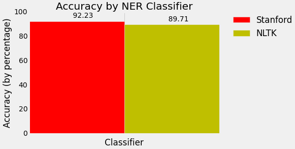
nltk_accuracy = accuracy(reference_annotations, nltk_formatted_prediction)
print(nltk_accuracy)

　　哇，准确率为.8971！

　　现在让我们测试斯坦福分类器。由于此分类器以元组形式生成输出，因此测试不需要更多的数据操作。

st = StanfordNERTagger('/usr/share/stanford-ner/classifiers/english.all.3class.distsim.crf.ser.gz',
                       '/usr/share/stanford-ner/stanford-ner.jar',
                       encoding='utf-8')                  
stanford_prediction = st.tag(pure_tokens)
stanford_accuracy = accuracy(reference_annotations, stanford_prediction)
print(stanford_accuracy)

　　.9223的准确率！更好！

　　如果你想绘制这个，这里有一些额外的代码。如果你想深入了解这如何工作，查看 matplotlib 系列：

import numpy as np
import matplotlib.pyplot as plt
from matplotlib import style

style.use('fivethirtyeight')

N = 1
ind = np.arange(N)  # the x locations for the groups
width = 0.35       # the width of the bars

fig, ax = plt.subplots()

stanford_percentage = stanford_accuracy * 100
rects1 = ax.bar(ind, stanford_percentage, width, color='r')

nltk_percentage = nltk_accuracy * 100
rects2 = ax.bar(ind+width, nltk_percentage, width, color='y')

# add some text for labels, title and axes ticks
ax.set_xlabel('Classifier')
ax.set_ylabel('Accuracy (by percentage)')
ax.set_title('Accuracy by NER Classifier')
ax.set_xticks(ind+width)
ax.set_xticklabels( ('') )

ax.legend( (rects1[0], rects2[0]), ('Stanford', 'NLTK'), bbox_to_anchor=(1.05, 1), loc=2, borderaxespad=0. )

def autolabel(rects):
    # attach some text labels
    for rect in rects:
        height = rect.get_height()
        ax.text(rect.get_x()+rect.get_width()/2., 1.02*height, '%10.2f' % float(height),
                ha='center', va='bottom')

autolabel(rects1)
autolabel(rects2)

plt.show()

二十六、测试 NLTK 和斯坦福 NER 标记器的速度

　　我们已经测试了我们的 NER 分类器的准确性，但是在决定使用哪个分类器时，还有更多的问题需要考虑。接下来我们来测试速度吧！

　　我们知道我们正在比较同一个东西，我们将在同一篇文章中进行测试。使用 NBC 新闻里的这个片段吧：

House Speaker John Boehner became animated Tuesday over the proposed Keystone Pipeline, castigating the Obama administration for not having approved the project yet.

Republican House Speaker John Boehner says there's "nothing complex about the Keystone Pipeline," and that it's time to build it.

"Complex? You think the Keystone Pipeline is complex?!" Boehner responded to a questioner. "It's been under study for five years! We build pipelines in America every day. Do you realize there are 200,000 miles of pipelines in the United States?"

The speaker went on: "And the only reason the president's involved in the Keystone Pipeline is because it crosses an international boundary. Listen, we can build it. There's nothing complex about the Keystone Pipeline -- it's time to build it."

Boehner said the president had no excuse at this point to not give the pipeline the go-ahead after the State Department released a report on Friday indicating the project would have a minimal impact on the environment.

Republicans have long pushed for construction of the project, which enjoys some measure of Democratic support as well. The GOP is considering conditioning an extension of the debt limit on approval of the project by Obama.

The White House, though, has said that it has no timetable for a final decision on the project.

　　首先，我们执行导入，通过阅读和分词来处理文章。

# -*- coding: utf-8 -*-

import nltk
import os
import numpy as np
import matplotlib.pyplot as plt
from matplotlib import style
from nltk import pos_tag
from nltk.tag import StanfordNERTagger
from nltk.tokenize import word_tokenize

style.use('fivethirtyeight')

# Process text  
def process_text(txt_file):
    raw_text = open("/usr/share/news_article.txt").read()
    token_text = word_tokenize(raw_text)
    return token_text

　　很棒！现在让我们写一些函数来拆分我们的分类任务。因为 NLTK NEG 分类器需要 POS 标签，所以我们会在我们的 NLTK 函数中加入 POS 标签。

# Stanford NER tagger    
def stanford_tagger(token_text):
    st = StanfordNERTagger('/usr/share/stanford-ner/classifiers/english.all.3class.distsim.crf.ser.gz',
                            '/usr/share/stanford-ner/stanford-ner.jar',
                            encoding='utf-8')   
    ne_tagged = st.tag(token_text)
    return(ne_tagged)
 
# NLTK POS and NER taggers   
def nltk_tagger(token_text):
    tagged_words = nltk.pos_tag(token_text)
    ne_tagged = nltk.ne_chunk(tagged_words)
    return(ne_tagged)

　　每个分类器都需要读取文章，并对命名实体进行分类，所以我们将这些函数包装在一个更大的函数中，使计时变得简单。

def stanford_main():
    print(stanford_tagger(process_text(txt_file)))

def nltk_main():
    print(nltk_tagger(process_text(txt_file)))

　　当我们调用我们的程序时，我们调用这些函数。我们将在os.times()函数调用中包装我们的stanford_main()和nltk_main()函数，取第四个索引，它是经过的时间。然后我们将图绘制我们的结果。

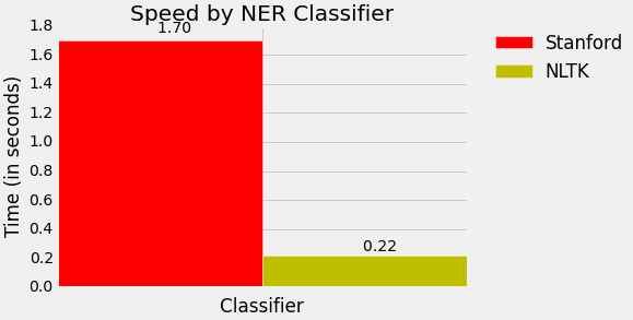
if __name__ == '__main__':
    stanford_t0 = os.times()[4]
    stanford_main()
    stanford_t1 = os.times()[4]
    stanford_total_time = stanford_t1 - stanford_t0
    
    nltk_t0 = os.times()[4]
    nltk_main()
    nltk_t1 = os.times()[4]
    nltk_total_time = nltk_t1 - nltk_t0
    
    time_plot(stanford_total_time, nltk_total_time)

　　对于我们的绘图，我们使用time_plot()函数：

def time_plot(stanford_total_time, nltk_total_time):
    N = 1
    ind = np.arange(N)  # the x locations for the groups
    width = 0.35       # the width of the bars
    stanford_total_time = stanford_total_time
    nltk_total_time = nltk_total_time   
    fig, ax = plt.subplots()    
    rects1 = ax.bar(ind, stanford_total_time, width, color='r')    
    rects2 = ax.bar(ind+width, nltk_total_time, width, color='y')
    
    # Add text for labels, title and axes ticks
    ax.set_xlabel('Classifier')
    ax.set_ylabel('Time (in seconds)')
    ax.set_title('Speed by NER Classifier')
    ax.set_xticks(ind+width)
    ax.set_xticklabels( ('') )   
    ax.legend( (rects1[0], rects2[0]), ('Stanford', 'NLTK'), bbox_to_anchor=(1.05, 1), loc=2, borderaxespad=0. )

    def autolabel(rects):
        # attach some text labels
        for rect in rects:
            height = rect.get_height()
            ax.text(rect.get_x()+rect.get_width()/2., 1.02*height, '%10.2f' % float(height),
                    ha='center', va='bottom')
    
    autolabel(rects1)
    autolabel(rects2)    
    plt.show()

　　哇，NLTK 像闪电一样快！看来斯坦福更准确，但 NLTK 更快。当平衡我们偏爱的精确度，和所需的计算资源时，这是需要知道的重要信息。

　　但是等等，还是有问题。我们的输出比较丑陋！这是斯坦福大学的一个小样本：

[('House', 'ORGANIZATION'), ('Speaker', 'O'), ('John', 'PERSON'), ('Boehner', 'PERSON'), ('became', 'O'), ('animated', 'O'), ('Tuesday', 'O'), ('over', 'O'), ('the', 'O'), ('proposed', 'O'), ('Keystone', 'ORGANIZATION'), ('Pipeline', 'ORGANIZATION'), (',', 'O'), ('castigating', 'O'), ('the', 'O'), ('Obama', 'PERSON'), ('administration', 'O'), ('for', 'O'), ('not', 'O'), ('having', 'O'), ('approved', 'O'), ('the', 'O'), ('project', 'O'), ('yet', 'O'), ('.', 'O')

　　以及 NLTK：

(S
  (ORGANIZATION House/NNP)
  Speaker/NNP
  (PERSON John/NNP Boehner/NNP)
  became/VBD
  animated/VBN
  Tuesday/NNP
  over/IN
  the/DT
  proposed/VBN
  (PERSON Keystone/NNP Pipeline/NNP)
  ,/,
  castigating/VBG
  the/DT
  (ORGANIZATION Obama/NNP)
  administration/NN
  for/IN
  not/RB
  having/VBG
  approved/VBN
  the/DT
  project/NN
  yet/RB
  ./.

　　让我们在下个教程中，将它们转为可读的形式。

二十七、使用 BIO 标签创建可读的命名实体列表

　　现在我们已经完成了测试，让我们将我们的命名实体转为良好的可读格式。

　　再次，我们将使用来自 NBC 新闻的同一篇新闻：

House Speaker John Boehner became animated Tuesday over the proposed Keystone Pipeline, castigating the Obama administration for not having approved the project yet.

Republican House Speaker John Boehner says there's "nothing complex about the Keystone Pipeline," and that it's time to build it.

"Complex? You think the Keystone Pipeline is complex?!" Boehner responded to a questioner. "It's been under study for five years! We build pipelines in America every day. Do you realize there are 200,000 miles of pipelines in the United States?"

The speaker went on: "And the only reason the president's involved in the Keystone Pipeline is because it crosses an international boundary. Listen, we can build it. There's nothing complex about the Keystone Pipeline -- it's time to build it."

Boehner said the president had no excuse at this point to not give the pipeline the go-ahead after the State Department released a report on Friday indicating the project would have a minimal impact on the environment.

Republicans have long pushed for construction of the project, which enjoys some measure of Democratic support as well. The GOP is considering conditioning an extension of the debt limit on approval of the project by Obama.

The White House, though, has said that it has no timetable for a final decision on the project.

　　我们的 NTLK 输出已经是树了（只需要最后一步），所以让我们来看看我们的斯坦福输出。我们将对标记进行 BIO 标记，B 分配给命名实体的开始，I 分配给内部，O 分配给其他。例如，如果我们的句子是Barack Obama went to Greece today，我们应该把它标记为Barack-B Obama-I went-O to-O Greece-B today-O。为此，我们将编写一系列条件来检查当前和以前的标记的O标签。

# -*- coding: utf-8 -*-

import nltk
import os
import numpy as np
import matplotlib.pyplot as plt
from matplotlib import style
from nltk import pos_tag
from nltk.tag import StanfordNERTagger
from nltk.tokenize import word_tokenize
from nltk.chunk import conlltags2tree
from nltk.tree import Tree

style.use('fivethirtyeight')

# Process text  
def process_text(txt_file):
    raw_text = open("/usr/share/news_article.txt").read()
    token_text = word_tokenize(raw_text)
    return token_text

# Stanford NER tagger    
def stanford_tagger(token_text):
    st = StanfordNERTagger('/usr/share/stanford-ner/classifiers/english.all.3class.distsim.crf.ser.gz',
                            '/usr/share/stanford-ner/stanford-ner.jar',
                            encoding='utf-8')   
    ne_tagged = st.tag(token_text)
    return(ne_tagged)
 
# NLTK POS and NER taggers   
def nltk_tagger(token_text):
    tagged_words = nltk.pos_tag(token_text)
    ne_tagged = nltk.ne_chunk(tagged_words)
    return(ne_tagged)

# Tag tokens with standard NLP BIO tags
def bio_tagger(ne_tagged):
        bio_tagged = []
        prev_tag = "O"
        for token, tag in ne_tagged:
            if tag == "O": #O
                bio_tagged.append((token, tag))
                prev_tag = tag
                continue
            if tag != "O" and prev_tag == "O": # Begin NE
                bio_tagged.append((token, "B-"+tag))
                prev_tag = tag
            elif prev_tag != "O" and prev_tag == tag: # Inside NE
                bio_tagged.append((token, "I-"+tag))
                prev_tag = tag
            elif prev_tag != "O" and prev_tag != tag: # Adjacent NE
                bio_tagged.append((token, "B-"+tag))
                prev_tag = tag
        return bio_tagged

　　现在我们将 BIO 标记后的标记写入树中，因此它们与 NLTK 输出格式相同。

# Create tree       
def stanford_tree(bio_tagged):
    tokens, ne_tags = zip(*bio_tagged)
    pos_tags = [pos for token, pos in pos_tag(tokens)]

    conlltags = [(token, pos, ne) for token, pos, ne in zip(tokens, pos_tags, ne_tags)]
    ne_tree = conlltags2tree(conlltags)
    return ne_tree

　　遍历并解析出所有命名实体：

# Parse named entities from tree
def structure_ne(ne_tree):
    ne = []
    for subtree in ne_tree:
        if type(subtree) == Tree: # If subtree is a noun chunk, i.e. NE != "O"
            ne_label = subtree.label()
            ne_string = " ".join([token for token, pos in subtree.leaves()])
            ne.append((ne_string, ne_label))
    return ne

　　在我们的调用中，我们把所有附加函数聚到一起。

def stanford_main():
    print(structure_ne(stanford_tree(bio_tagger(stanford_tagger(process_text(txt_file))))))

def nltk_main():
    print(structure_ne(nltk_tagger(process_text(txt_file))))

　　之后调用这些函数：

if __name__ == '__main__':
    stanford_main()
    nltk_main()

　　这里是来自斯坦福的看起来不错的输出：

[('House', 'ORGANIZATION'), ('John Boehner', 'PERSON'), ('Keystone Pipeline', 'ORGANIZATION'), ('Obama', 'PERSON'), ('Republican House', 'ORGANIZATION'), ('John Boehner', 'PERSON'), ('Keystone Pipeline', 'ORGANIZATION'), ('Keystone Pipeline', 'ORGANIZATION'), ('Boehner', 'PERSON'), ('America', 'LOCATION'), ('United States', 'LOCATION'), ('Keystone Pipeline', 'ORGANIZATION'), ('Keystone Pipeline', 'ORGANIZATION'), ('Boehner', 'PERSON'), ('State Department', 'ORGANIZATION'), ('Republicans', 'MISC'), ('Democratic', 'MISC'), ('GOP', 'MISC'), ('Obama', 'PERSON'), ('White House', 'LOCATION')]

　　以及来自 NLTK 的：

[('House', 'ORGANIZATION'), ('John Boehner', 'PERSON'), ('Keystone Pipeline', 'PERSON'), ('Obama', 'ORGANIZATION'), ('Republican', 'ORGANIZATION'), ('House', 'ORGANIZATION'), ('John Boehner', 'PERSON'), ('Keystone Pipeline', 'ORGANIZATION'), ('Keystone Pipeline', 'ORGANIZATION'), ('Boehner', 'PERSON'), ('America', 'GPE'), ('United States', 'GPE'), ('Keystone Pipeline', 'ORGANIZATION'), ('Listen', 'PERSON'), ('Keystone', 'ORGANIZATION'), ('Boehner', 'PERSON'), ('State Department', 'ORGANIZATION'), ('Democratic', 'ORGANIZATION'), ('GOP', 'ORGANIZATION'), ('Obama', 'PERSON'), ('White House', 'FACILITY')]

分块在一起，可读性强。

注：参考：Natural Language Process

posted on 2019-09-04 13:18 农夫三拳有點疼阅读(21008) 评论(3) 编辑收藏举报

会员力量，点亮园子希望

刷新页面返回顶部

农夫三拳有點疼

NLTK最详细功能介绍

目录

四、NLTK 与停止词

五、NLTK 词干提取

六、NLTK 词性标注

七、NLTK 分块

八、 NLTK 添加缝隙（Chinking）

九、NLTK 命名实体识别

十、NLTK 词形还原

十一、NLTK 语料库

十二、 NLTK 和 Wordnet

十三、NLTK 文本分类

十四、使用 NLTK 将单词转换为特征

十五、NLTK 朴素贝叶斯分类器

十六、使用 NLTK 保存分类器

十七、NLTK 和 Sklearn

十八、使用 NLTK 组合算法

十九、使用 NLTK 调查偏差

二十、使用 NLTK 改善情感分析的训练数据

二十一、使用 NLTK 为情感分析创建模块

二十二、NLTK Twitter 情感分析

二十三，使用 NLTK 绘制 Twitter 实时情感分析

二十四、斯坦福 NER 标记器与命名实体识别

二十五、测试 NLTK 和斯坦福 NER 标记器的准确性

二十六、测试 NLTK 和斯坦福 NER 标记器的速度

二十七、使用 BIO 标签创建可读的命名实体列表

一、前言

二、NLTK模块

四、NLTK 与停止词

五、NLTK 词干提取

六、NLTK 词性标注

七、NLTK 分块

八、 NLTK 添加缝隙（Chinking）

九、NLTK 命名实体识别

十、NLTK 词形还原

十一、 NLTK 语料库

十二、NLTK 和 Wordnet

十三、NLTK 文本分类

十四、使用 NLTK 将单词转换为特征

十五、NLTK 朴素贝叶斯分类器

十六、使用 NLTK 保存分类器

十七、NLTK 和 Sklearn

十八、使用 NLTK 组合算法

十九、使用 NLTK 调查偏差

二十、使用 NLTK 改善情感分析的训练数据

二十一、使用 NLTK 为情感分析创建模块

二十二、NLTK Twitter 情感分析

二十三，使用 NLTK 绘制 Twitter 实时情感分析

二十四、斯坦福 NER 标记器与命名实体识别

二十五、测试 NLTK 和斯坦福 NER 标记器的准确性

二十六、测试 NLTK 和斯坦福 NER 标记器的速度

二十七、使用 BIO 标签创建可读的命名实体列表

导航

一、前言　