autograd实现线性回归

In [1]:
import torch as t
from torch.autograd import Variable as V
from matplotlib import pyplot as plt
from IPython import display
In [2]:
# 为了在不同计算机上运行时下面输出的结果一致,设置随机数种子
t.manual_seed(1000)

def get_fake_data(batch_size=8):
    """
    //产生随机数:y = x*2 + 3,加上噪声
    """
    x = t.rand(batch_size, 1) * 20
    y = x * 2 + (1 + t.randn(batch_size, 1)) * 3
    return x , y
In [3]:
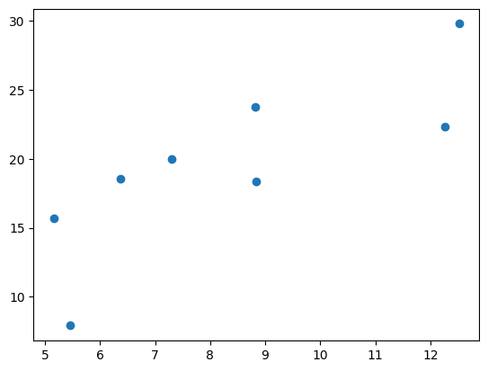
# 查看x-y的分布情况
x, y = get_fake_data()
plt.scatter(x.squeeze().numpy(), y.squeeze().numpy())
Out[3]:
<matplotlib.collections.PathCollection at 0x24972bf5508>
In [4]:
# 初始化随机参数
w = V(t.rand(1, 1), requires_grad=True)
b = V(t.zeros(1, 1), requires_grad=True)
# 设置学习率
lr = 0.001
In [5]:
for ii in range(2000):
    x, y = get_fake_data()
    x, y = V(x), V(y)

    # forward:计算loss
    y_pred = x.mm(w) + b.expand_as(y)
    loss = 0.5 * (y_pred - y) ** 2
    loss = loss.sum()

    # backward:自动计算梯度
    loss.backward()

    # 更新参数
    w.data.sub_(lr * w.grad.data)
    b.data.sub_(lr * b.grad.data)

    # 梯度清零
    w.grad.data.zero_()
    b.grad.data.zero_()

    if ii%2000 == 0:
        # 画图
        display.clear_output(wait=True)
        x = t.arange(0, 20).view(-1, 1)
        y = x.mm(w.data.long()) + b.data.expand_as(x)
        # predicted
        plt.plot(x.numpy(), y.numpy())

        x2, y2 = get_fake_data(batch_size=20)
        # true data
        plt.scatter(x2.numpy(), y2.numpy())

        plt.xlim(0, 20)
        plt.ylim(0, 41)
        plt.show()
        plt.pause(0.5)
print(w.item(), b.item())
2.054152727127075 3.0143353939056396

 浙公网安备 33010602011771号