线性回归
In [1]:
import torch as t
%matplotlib inline
from matplotlib import pyplot as plt
from IPython import display
In [2]:
# 设置随机种子,保证在不同计算机上运行时下面的输出一致
t.manual_seed(1000)
def get_fake_data(batch_size=8):
    """
    //产生随机数据:y = x*2+3,加上一些噪声
    """
    x = t.rand(batch_size, 1) * 20
    y = x * 2 + (1 + t.randn(batch_size, 1) )* 3
    return x , y
In [3]:
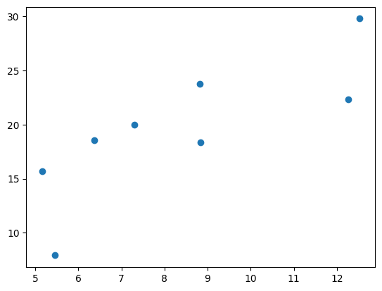
# 查看产生的x-y分布
x , y = get_fake_data()
plt.scatter(x.squeeze().numpy(),y.squeeze().numpy())
Out[3]:
<matplotlib.collections.PathCollection at 0x1c54aa25488>
In [4]:
# 随机初始话参数
w = t.rand(1, 1)
b = t.zeros(1, 1)
In [5]:
lr=0.001#学习率
for ii in range(2000):
x, y = get_fake_data()
#forward:计算loss
y_pred = x.mm(w)+b.expand_as(y)
loss = 0.5 * (y_pred - y) ** 2 #均方误差
loss = loss.sum()
#backward:手动计算梯度
dloss = 1
dy_pred = dloss * (y_pred - y)
dw = x.t().mm(dy_pred)
db = dy_pred.sum()
#更新参数
w.sub_(lr * dw)
b.sub_(lr * db)
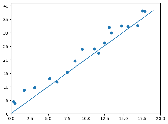
if (ii % 2000) == 0:
#画图
display.clear_output (wait=True)
x = t.arange(0, 20).view(-1,1)
y = x.mm(w.data.long()) + b.expand_as(x)
plt.plot(x.numpy(),y.numpy())
#预测
x2,y2 = get_fake_data(batch_size=20)
plt.scatter(x2.numpy (),y2.numpy()) #true data
plt.xlim(0,20)
plt.ylim(0,41)
plt.show()
plt.pause(0.5)
In [6]:
# 当前w与b
print(w.item(), b.item())
2.054126262664795 3.014718770980835

 浙公网安备 33010602011771号