
R语言与概率统计(六) 主成分分析 因子分析

超高维度分析,N*P的矩阵,N为样本个数,P为指标,N<<P
PCA:抓住对y对重要的影响因素
主要有三种:PCA,因子分析,回归方程+惩罚函数(如LASSO)
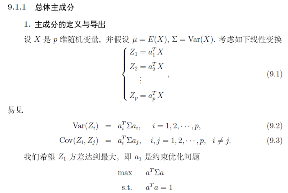

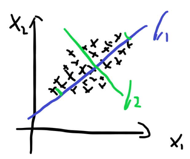
为了降维,用更少的变量解决问题,如果是二维的,那么就是找到一条线,要使这些点再线上的投影最大,投影最大,就是越分散,就考虑方差最大。


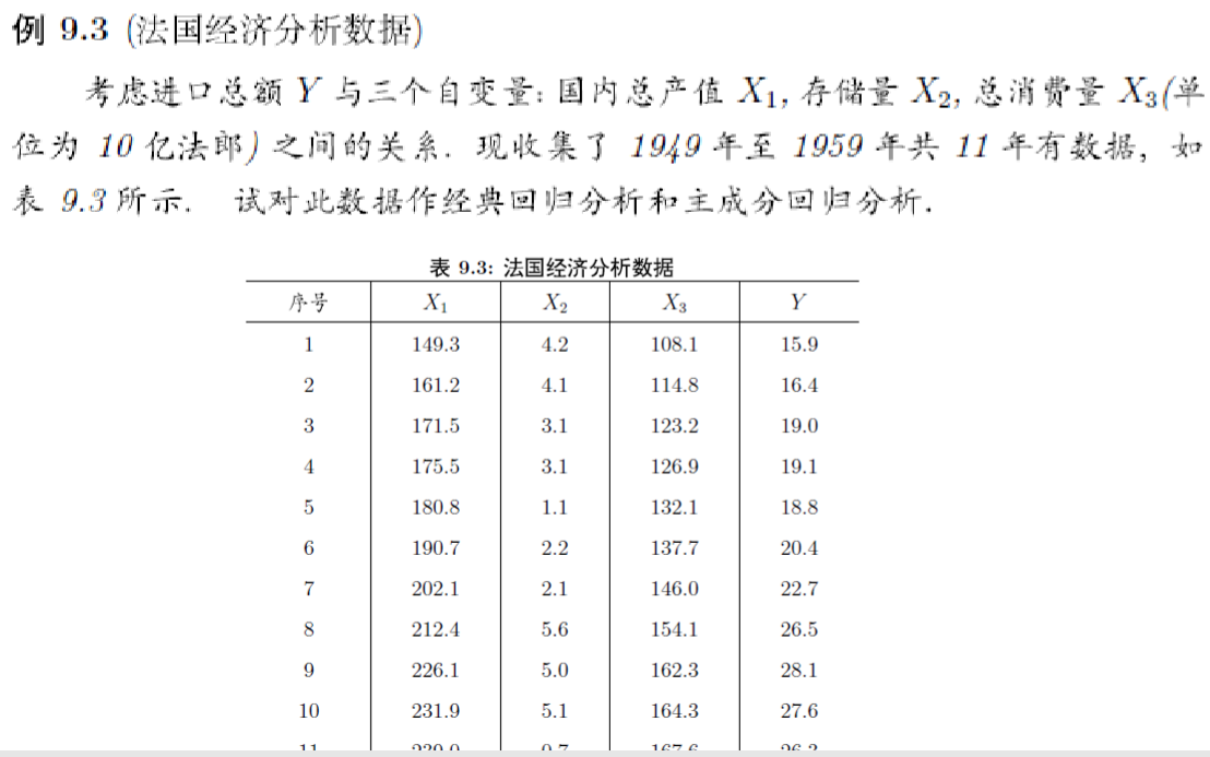


> conomy<-data.frame(
+ x1=c(149.3, 161.2, 171.5, 175.5, 180.8, 190.7,
+ 202.1, 212.4, 226.1, 231.9, 239.0),
+ x2=c(4.2, 4.1, 3.1, 3.1, 1.1, 2.2, 2.1, 5.6, 5.0, 5.1, 0.7),
+ x3=c(108.1, 114.8, 123.2, 126.9, 132.1, 137.7,
+ 146.0, 154.1, 162.3, 164.3, 167.6),
+ y=c(15.9, 16.4, 19.0, 19.1, 18.8, 20.4, 22.7,
+ 26.5, 28.1, 27.6, 26.3)
+ )
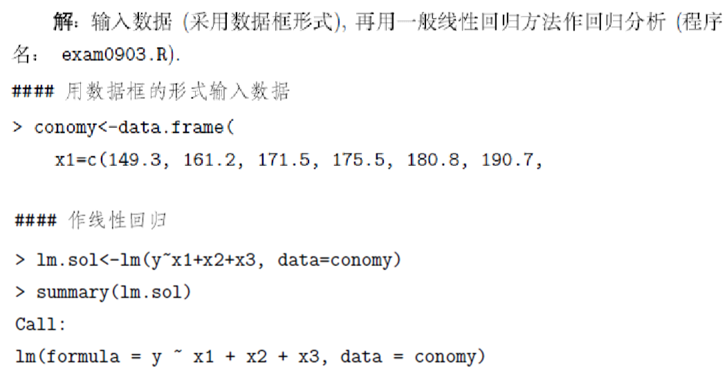
> #### 作线性回归
> lm.sol<-lm(y~x1+x2+x3, data=conomy)
> summary(lm.sol)
Call:
lm(formula = y ~ x1 + x2 + x3, data = conomy)
Residuals:
Min 1Q Median 3Q Max
-0.52367 -0.38953 0.05424 0.22644 0.78313
Coefficients:
Estimate Std. Error t value Pr(>|t|)
(Intercept) -10.12799 1.21216 -8.355 6.9e-05 ***
x1 -0.05140 0.07028 -0.731 0.488344
x2 0.58695 0.09462 6.203 0.000444 ***
x3 0.28685 0.10221 2.807 0.026277 *
---
Signif. codes: 0 ‘***’ 0.001 ‘**’ 0.01 ‘*’ 0.05 ‘.’ 0.1 ‘ ’ 1
Residual standard error: 0.4889 on 7 degrees of freedom
Multiple R-squared: 0.9919, Adjusted R-squared: 0.9884
F-statistic: 285.6 on 3 and 7 DF, p-value: 1.112e-07
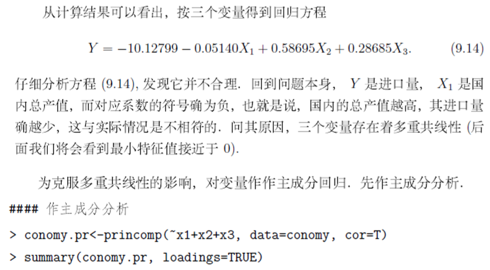
> #### 作主成分分析
> conomy.pr<-princomp(~x1+x2+x3, data=conomy, cor=T)
> summary(conomy.pr, loadings=TRUE)
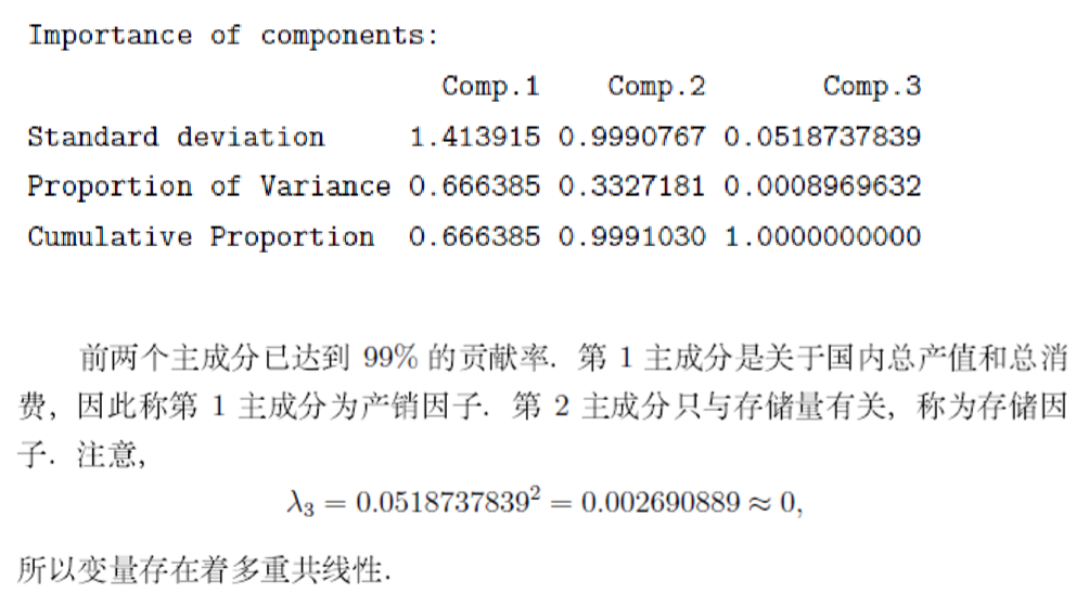
Importance of components:
Comp.1 Comp.2 Comp.3
Standard deviation 1.413915 0.9990767 0.0518737839
Proportion of Variance 0.666385 0.3327181 0.0008969632
Cumulative Proportion 0.666385 0.9991030 1.0000000000
Loadings:
Comp.1 Comp.2 Comp.3
x1 0.706 0.707
x2 -0.999
x3 0.707 -0.707
> #### 预测测样本主成分, 并作主成分分析
> pre<-predict(conomy.pr)
> conomy$z1<-pre[,1]
> conomy$z2<-pre[,2]
> lm.sol<-lm(y~z1+z2, data=conomy)
> summary(lm.sol)
Call:
lm(formula = y ~ z1 + z2, data = conomy)
Residuals:
Min 1Q Median 3Q Max
-0.89838 -0.26050 0.08435 0.35677 0.66863
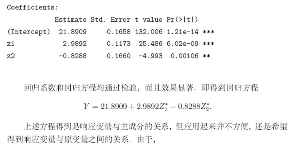
Coefficients:
Estimate Std. Error t value Pr(>|t|)
(Intercept) 21.8909 0.1658 132.006 1.21e-14 ***
z1 2.9892 0.1173 25.486 6.02e-09 ***
z2 -0.8288 0.1660 -4.993 0.00106 **
---
Signif. codes: 0 ‘***’ 0.001 ‘**’ 0.01 ‘*’ 0.05 ‘.’ 0.1 ‘ ’ 1
Residual standard error: 0.55 on 8 degrees of freedom
Multiple R-squared: 0.9883, Adjusted R-squared: 0.9853
F-statistic: 337.2 on 2 and 8 DF, p-value: 1.888e-08
> #### 作变换, 得到原坐标下的关系表达式
> beta<-coef(lm.sol); A<-loadings(conomy.pr)
> x.bar<-conomy.pr$center; x.sd<-conomy.pr$scale
> coef<-(beta[2]*A[,1]+ beta[3]*A[,2])/x.sd
> beta0 <- beta[1]- sum(x.bar * coef)
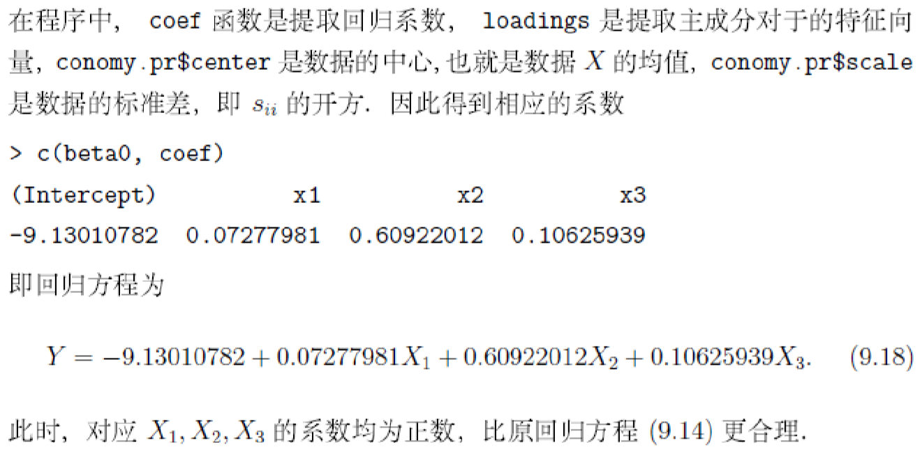
> c(beta0, coef)
(Intercept) x1 x2 x3
-9.13010782 0.07277981 0.60922012 0.10625939


 浙公网安备 33010602011771号