Matlab建立系统模型实验

Matlab建立系统模型实验

第一题

>> num=[1,2];
>> den=[1 1 10];
>> sys=tf(num,den)

sys =
 
     s + 2
  ------------
  s^2 + s + 10
 
Continuous-time transfer function.

>> syszpk=zpk(sys)

syszpk =
 
      (s+2)
  --------------
  (s^2 + s + 10)
 
Continuous-time zero/pole/gain model.

第二题

>> z=-2;
>> p=[-0.4 -15 -25];
>> k=18;
>> sys=zpk(z,p,k)

sys =
 
        18 (s+2)
  ---------------------
  (s+0.4) (s+15) (s+25)
 
Continuous-time zero/pole/gain model.

第三题

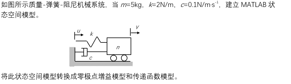
>> m=5;k=2;c=0.1;
>> A=[0,1;-k/m,-c/m];
>> B=[0,k/m]';
>> C=[1,0];
>> D=0;
>> sys=ss(A,B,C,D)

sys =
 
  A = 
          x1     x2
   x1      0      1
   x2   -0.4  -0.02
 
  B = 
        u1
   x1    0
   x2  0.4
 
  C = 
       x1  x2
   y1   1   0
 
  D = 
       u1
   y1   0
 
Continuous-time state-space model.

第四题

>> NUM=[5,3];
>> DEN=[1,6,11,6];
>> SYS=tf(NUM,DEN,'Inputdelay',0.5)

SYS =
 
                       5 s + 3
  exp(-0.5*s) * ----------------------
                s^3 + 6 s^2 + 11 s + 6
 
Continuous-time transfer function.

>> NUM=[5,3];
>> DEN=[1,6,11,6];
>> SYS=tf(NUM,DEN,'Outputdelay',0.5)

SYS =
 
                       5 s + 3
  exp(-0.5*s) * ----------------------
                s^3 + 6 s^2 + 11 s + 6
 
Continuous-time transfer function.

第五题

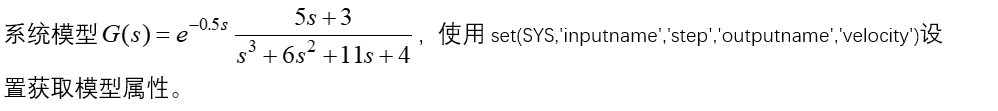
>> NUM=[5,3];DEN=[1,6,11,4];
>> SYS=tf(NUM,DEN,'Inputdelay',0.5);
>> set(SYS,'inputname','step','outputname','velocity')
>> SYS

SYS =
 
  From input "step" to output "velocity":
                       5 s + 3
  exp(-0.5*s) * ----------------------
                s^3 + 6 s^2 + 11 s + 4
 
Continuous-time transfer function.

>> get(SYS)
       Numerator: {[0 0 5 3]}
     Denominator: {[1 6 11 4]}
        Variable: 's'
         IODelay: 0
      InputDelay: 0.5000
     OutputDelay: 0
              Ts: 0
        TimeUnit: 'seconds'
       InputName: {'step'}
       InputUnit: {''}
      InputGroup: [1×1 struct]
      OutputName: {'velocity'}
      OutputUnit: {''}
     OutputGroup: [1×1 struct]
           Notes: [0×1 string]
        UserData: []
            Name: ''
    SamplingGrid: [1×1 struct]

第六题

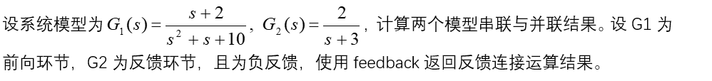
>> sys1=tf([1,2],[1,1,10]);
>> sys2=zpk([],-3,2);
>> sys=feedback(sys1,sys2,-1)

sys =
 
            (s+3) (s+2)
  --------------------------------
  (s+2.885) (s^2 + 1.115s + 11.78)
 
Continuous-time zero/pole/gain model.

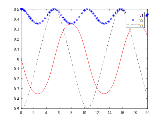
第七题

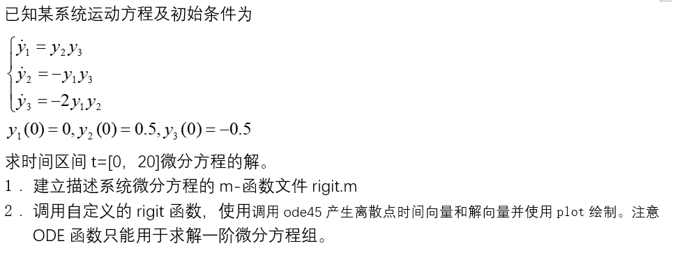
function dy=rigit(t,y)
dy=zeros(3,1);
dy(1)=y(2)*y(3);
dy(2)=-y(1)*y(3);
dy(3)=-2*y(1)*y(2);

>> [T,y]=ode45('rigit',[0,20],[0,0.5,-0.5]);
>> plot(T,y(:,1),'r',T,y(:,2),'b*',T,y(:,3),'k-.')
>> legend('y1','y2','y3')

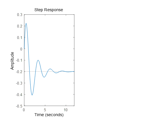
第八题

>> sys=tf([1,-1],[1,1.5]);
>> sys=tf([1,-1],[1,1,5]);
>> subplot(1,2,1),step(sys,20)
>> subplot(1,2,1),step(sys)

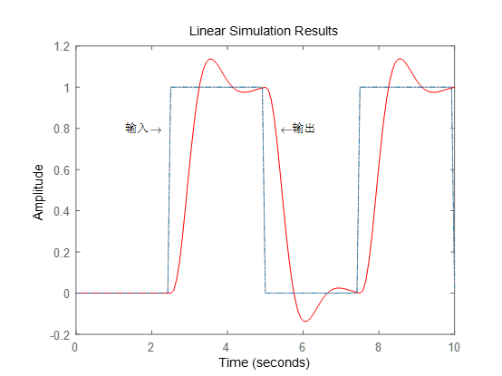
第九题

>> sys=tf([3,100],[1,10,40,100]);
>> [u,t]=gensig('square',5,10);
>> lsim(sys,'r',u,t)
>> hold on
>> plot(t,u,'-.')
>> hold off
>> text(1.3,0.8,'输入\rightarrow')
>> text(5.4,0.8,'\leftarrow输出')

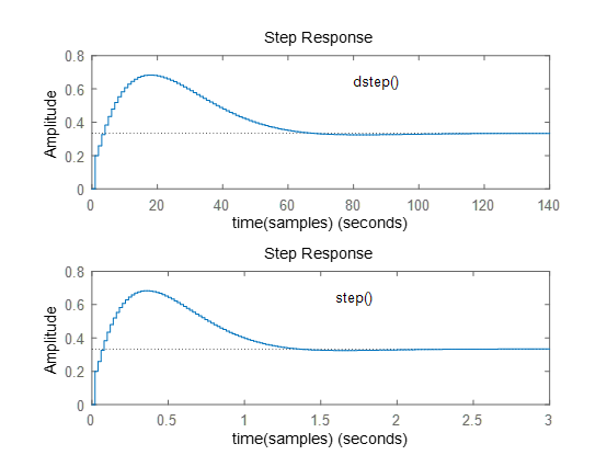
第十题

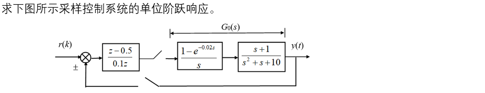
>> G1=tf([1,1],[1 1 10]);
>> G0=c2d(G1,0.02,'zoh');
>> Gc=tf([1 -0.5],[0.1 0],0.02);
>> Wz=G0*Gc/(1+G0*Gc);
>> [num,den]=tfdata(Wz,'v');
>> subplot(2,1,1),dstep(num,den)
>> xlabel('time(samples)')
>> text(80,0.65,'dstep()')
>> subplot(2,1,2),step(Wz)
>> xlabel('time(samples)')
>> text(1.6,0.65,'step()')

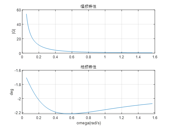
第十一题

>> num=[11 11];den=[1 15 4 0];
>> w=0.05:0.01:0.5*pi;
>> Gw=polyval(num,j*w)./polyval(den,j*w);
>> mag=abs(Gw);
>> theta=angle(Gw);
>> subplot(2,1,1),plot(w,mag)
>> grid,title('幅频特性')
>> ylabel('|G|')
>> subplot(2,1,2),plot(w,theta)
>> grid,title('相频特性')
>> xlabel('omega(rad/s)'),ylabel('deg')

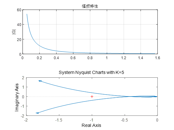
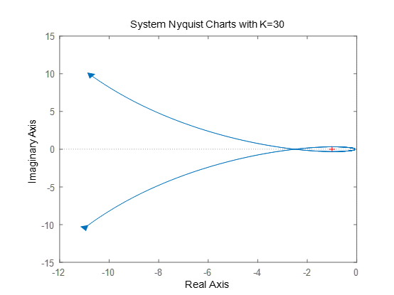
第十二题

>> w=linspace(0.5,5,1000)*pi;
>> sys1=zpk([],[0 -10 -2],100);
>> sys2=zpk([],[0 -10 -2],600);
>> figure(1)
>> nyquist(sys1,w);
>> title('System Nyquist Charts with K=5')
>> figure(2)
>> nyquist(sys2,w)
>> title('System Nyquist Charts with K=30')

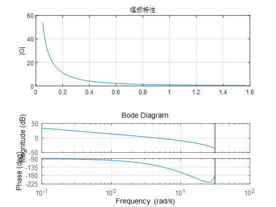
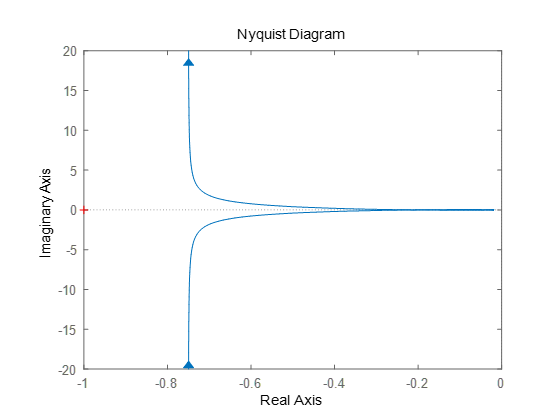
第十三题

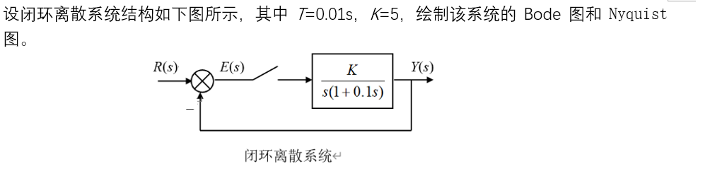
>> Ts=0.1;K=5;
>> Gs=zpk([],[0,-10],K*10);
>> Gz=c2d(Gs,Ts,'zoh');
>> [num,den,Ts]=tfdata(Gz,'v');
>> figure(1)
>> dbode(num,den,Ts)
>> grid,figure(2)
>> dnyquist(num,den,Ts)