MLPClassifier 隐藏层不包括输入和输出

多层感知机（MLP）原理简介

多层感知机（MLP，Multilayer Perceptron）也叫人工神经网络（ANN，Artificial Neural Network），除了输入输出层，它中间可以有多个隐层，最简单的MLP只含一个隐层，即三层的结构，如下图：

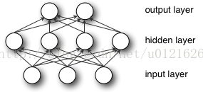
从上图可以看到，多层感知机层与层之间是全连接的（全连接的意思就是：上一层的任何一个神经元与下一层的所有神经元都有连接）。多层感知机最底层是输入层，中间是隐藏层，最后是输出层。

输入层没什么好说，你输入什么就是什么，比如输入是一个n维向量，就有n个神经元。

隐藏层的神经元怎么得来？首先它与输入层是全连接的，假设输入层用向量X表示，则隐藏层的输出就是

f(W1X+b1)，W1是权重（也叫连接系数），b1是偏置，函数f 可以是常用的sigmoid函数或者tanh函数：

最后就是输出层，输出层与隐藏层是什么关系？其实隐藏层到输出层可以看成是一个多类别的逻辑回归，也即softmax回归，所以输出层的输出就是softmax(W2X1+b2)，X1表示隐藏层的输出f(W1X+b1)。

`sklearn.neural_network`.MLPClassifier

class sklearn.neural_network.MLPClassifier(hidden_layer_sizes=(100, ), activation=’relu’, solver=’adam’, alpha=0.0001, batch_size=’auto’, learning_rate=’constant’, learning_rate_init=0.001, power_t=0.5, max_iter=200, shuffle=True, random_state=None, tol=0.0001, verbose=False, warm_start=False, momentum=0.9, nesterovs_momentum=True, early_stopping=False, validation_fraction=0.1, beta_1=0.9, beta_2=0.999, epsilon=1e-08, n_iter_no_change=10)[source]

Multi-layer Perceptron classifier.

This model optimizes the log-loss function using LBFGS or stochastic gradient descent.

New in version 0.18.

Parameters:

Parameters:	hidden_layer_sizes : tuple, length = n_layers - 2, default (100,) The ith element represents the number of neurons in the ith hidden layer. activation : {‘identity’, ‘logistic’, ‘tanh’, ‘relu’}, default ‘relu’ Activation function for the hidden layer. ‘identity’, no-op activation, useful to implement linear bottleneck, returns f(x) = x ‘logistic’, the logistic sigmoid function, returns f(x) = 1 / (1 + exp(-x)). ‘tanh’, the hyperbolic tan function, returns f(x) = tanh(x). ‘relu’, the rectified linear unit function, returns f(x) = max(0, x) solver : {‘lbfgs’, ‘sgd’, ‘adam’}, default ‘adam’ The solver for weight optimization. ‘lbfgs’ is an optimizer in the family of quasi-Newton methods. ‘sgd’ refers to stochastic gradient descent. ‘adam’ refers to a stochastic gradient-based optimizer proposed by Kingma, Diederik, and Jimmy Ba Note: The default solver ‘adam’ works pretty well on relatively large datasets (with thousands of training samples or more) in terms of both training time and validation score. For small datasets, however, ‘lbfgs’ can converge faster and perform better. alpha : float, optional, default 0.0001 L2 penalty (regularization term) parameter. batch_size : int, optional, default ‘auto’ Size of minibatches for stochastic optimizers. If the solver is ‘lbfgs’, the classifier will not use minibatch. When set to “auto”, batch_size=min(200, n_samples) learning_rate : {‘constant’, ‘invscaling’, ‘adaptive’}, default ‘constant’ Learning rate schedule for weight updates. ‘constant’ is a constant learning rate given by ‘learning_rate_init’. ‘invscaling’ gradually decreases the learning rate `learning_rate_` at each time step ‘t’ using an inverse scaling exponent of ‘power_t’. effective_learning_rate = learning_rate_init / pow(t, power_t) ‘adaptive’ keeps the learning rate constant to ‘learning_rate_init’ as long as training loss keeps decreasing. Each time two consecutive epochs fail to decrease training loss by at least tol, or fail to increase validation score by at least tol if ‘early_stopping’ is on, the current learning rate is divided by 5. Only used when `solver='sgd'`. learning_rate_init : double, optional, default 0.001 The initial learning rate used. It controls the step-size in updating the weights. Only used when solver=’sgd’ or ‘adam’. power_t : double, optional, default 0.5 The exponent for inverse scaling learning rate. It is used in updating effective learning rate when the learning_rate is set to ‘invscaling’. Only used when solver=’sgd’.

hidden_layer_sizes : tuple, length = n_layers - 2, default (100,)

The ith element represents the number of neurons in the ith hidden layer.

activation : {‘identity’, ‘logistic’, ‘tanh’, ‘relu’}, default ‘relu’

Activation function for the hidden layer.

‘identity’, no-op activation, useful to implement linear bottleneck, returns f(x) = x
‘logistic’, the logistic sigmoid function, returns f(x) = 1 / (1 + exp(-x)).
‘tanh’, the hyperbolic tan function, returns f(x) = tanh(x).
‘relu’, the rectified linear unit function, returns f(x) = max(0, x)

solver : {‘lbfgs’, ‘sgd’, ‘adam’}, default ‘adam’

The solver for weight optimization.

‘lbfgs’ is an optimizer in the family of quasi-Newton methods.
‘sgd’ refers to stochastic gradient descent.
‘adam’ refers to a stochastic gradient-based optimizer proposed by Kingma, Diederik, and Jimmy Ba

Note: The default solver ‘adam’ works pretty well on relatively large datasets (with thousands of training samples or more) in terms of both training time and validation score. For small datasets, however, ‘lbfgs’ can converge faster and perform better.

alpha : float, optional, default 0.0001

L2 penalty (regularization term) parameter.

batch_size : int, optional, default ‘auto’

Size of minibatches for stochastic optimizers. If the solver is ‘lbfgs’, the classifier will not use minibatch. When set to “auto”, batch_size=min(200, n_samples)

learning_rate : {‘constant’, ‘invscaling’, ‘adaptive’}, default ‘constant’

Learning rate schedule for weight updates.

‘constant’ is a constant learning rate given by ‘learning_rate_init’.
‘invscaling’ gradually decreases the learning rate learning_rate_ at each time step ‘t’ using an inverse scaling exponent of ‘power_t’. effective_learning_rate = learning_rate_init / pow(t, power_t)
‘adaptive’ keeps the learning rate constant to ‘learning_rate_init’ as long as training loss keeps decreasing. Each time two consecutive epochs fail to decrease training loss by at least tol, or fail to increase validation score by at least tol if ‘early_stopping’ is on, the current learning rate is divided by 5.

Only used when solver='sgd'.

learning_rate_init : double, optional, default 0.001

The initial learning rate used. It controls the step-size in updating the weights. Only used when solver=’sgd’ or ‘adam’.

power_t : double, optional, default 0.5

The exponent for inverse scaling learning rate. It is used in updating effective learning rate when the learning_rate is set to ‘invscaling’. Only used when solver=’sgd’.

概述

以监督学习为例，假设我们有训练样本集 $\textstyle (x(^ i),y(^ i))$ ，那么神经网络算法能够提供一种复杂且非线性的假设模型 $\textstyle h_{W,b}(x)$ ，它具有参数 $\textstyle W, b$ ，可以以此参数来拟合我们的数据。

为了描述神经网络，我们先从最简单的神经网络讲起，这个神经网络仅由一个“神经元”构成，以下即是这个“神经元”的图示：

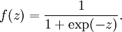
这个“神经元”是一个以 $\textstyle x_1, x_2, x_3$ 及截距 $\textstyle +1$ 为输入值的运算单元，其输出为 $\textstyle h_{W,b}(x) = f(W^Tx) = f(\sum_{i=1}^3 W_{i}x_i +b)$ ，其中函数 $\textstyle f : \Re \mapsto \Re$ 被称为“激活函数”。在本教程中，我们选用sigmoid函数作为激活函数 $\textstyle f(\cdot)$

$f(z) = \frac{1}{1+\exp(-z)}.$

可以看出，这个单一“神经元”的输入－输出映射关系其实就是一个逻辑回归（logistic regression）。

虽然本系列教程采用sigmoid函数，但你也可以选择双曲正切函数（tanh）：

$f(z) = \tanh(z) = \frac{e^z - e^{-z}}{e^z + e^{-z}},$

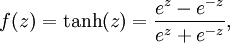
以下分别是sigmoid及tanh的函数图像

$\textstyle \tanh(z)$ 函数是sigmoid函数的一种变体，它的取值范围为 $\textstyle [-1,1]$ ，而不是sigmoid函数的 $\textstyle [0,1]$ 。

注意，与其它地方（包括OpenClassroom公开课以及斯坦福大学CS229课程）不同的是，这里我们不再令 $\textstyle x_0=1$ 。取而代之，我们用单独的参数 $\textstyle b$ 来表示截距。

最后要说明的是，有一个等式我们以后会经常用到：如果选择 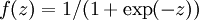$\textstyle f(z) = 1/(1+\exp(-z))$ ，也就是sigmoid函数，那么它的导数就是 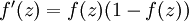$\textstyle f'(z) = f(z) (1-f(z))$ （如果选择tanh函数，那它的导数就是 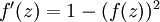$\textstyle f'(z) = 1- (f(z))^2$ ，你可以根据sigmoid（或tanh）函数的定义自行推导这个等式。

神经网络模型

所谓神经网络就是将许多个单一“神经元”联结在一起，这样，一个“神经元”的输出就可以是另一个“神经元”的输入。例如，下图就是一个简单的神经网络：

我们使用圆圈来表示神经网络的输入，标上“ $\textstyle +1$ ”的圆圈被称为偏置节点，也就是截距项。神经网络最左边的一层叫做输入层，最右的一层叫做输出层（本例中，输出层只有一个节点）。中间所有节点组成的一层叫做隐藏层，因为我们不能在训练样本集中观测到它们的值。同时可以看到，以上神经网络的例子中有3个输入单元（偏置单元不计在内），3个隐藏单元及一个输出单元。

我们用 $\textstyle {n}_l$ 来表示网络的层数，本例中 $\textstyle n_l=3$ ，我们将第 $\textstyle l$ 层记为 $\textstyle L_l$ ，于是 $\textstyle L_1$ 是输入层，输出层是 $\textstyle L_{n_l}$ 。本例神经网络有参数 $\textstyle (W,b) = (W^{(1)}, b^{(1)}, W^{(2)}, b^{(2)})$ ，其中 $\textstyle W^{(l)}_{ij}$ （下面的式子中用到）是第 $\textstyle l$ 层第 $\textstyle j$ 单元与第 $\textstyle l+1$ 层第 $\textstyle i$ 单元之间的联接参数（其实就是连接线上的权重，注意标号顺序）， $\textstyle b^{(l)}_i$ 是第 $\textstyle l+1$ 层第 $\textstyle i$ 单元的偏置项。因此在本例中， $\textstyle W^{(1)} \in \Re^{3\times 3}$ ， $\textstyle W^{(2)} \in \Re^{1\times 3}$ 。注意，没有其他单元连向偏置单元(即偏置单元没有输入)，因为它们总是输出 $\textstyle +1$ 。同时，我们用 $\textstyle s_l$ 表示第 $\textstyle l$ 层的节点数（偏置单元不计在内）。

我们用 $\textstyle a^{(l)}_i$ 表示第 $\textstyle l$ 层第 $\textstyle i$ 单元的激活值（输出值）。当 $\textstyle l=1$ 时， $\textstyle a^{(1)}_i = x_i$ ，也就是第 $\textstyle i$ 个输入值（输入值的第 $\textstyle i$ 个特征）。对于给定参数集合 $\textstyle W,b$ ，我们的神经网络就可以按照函数 $\textstyle h_{W,b}(x)$ 来计算输出结果。本例神经网络的计算步骤如下：

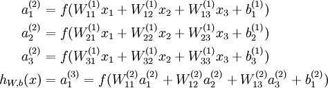
$\begin{align} a_1^{(2)} &= f(W_{11}^{(1)}x_1 + W_{12}^{(1)} x_2 + W_{13}^{(1)} x_3 + b_1^{(1)}) \\ a_2^{(2)} &= f(W_{21}^{(1)}x_1 + W_{22}^{(1)} x_2 + W_{23}^{(1)} x_3 + b_2^{(1)}) \\ a_3^{(2)} &= f(W_{31}^{(1)}x_1 + W_{32}^{(1)} x_2 + W_{33}^{(1)} x_3 + b_3^{(1)}) \\ h_{W,b}(x) &= a_1^{(3)} = f(W_{11}^{(2)}a_1^{(2)} + W_{12}^{(2)} a_2^{(2)} + W_{13}^{(2)} a_3^{(2)} + b_1^{(2)}) \end{align}$

我们用 $\textstyle z^{(l)}_i$ 表示第 $\textstyle l$ 层第 $\textstyle i$ 单元输入加权和（包括偏置单元），比如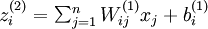， $\textstyle z_i^{(2)} = \sum_{j=1}^n W^{(1)}_{ij} x_j + b^{(1)}_i$ ，则 $\textstyle a^{(l)}_i = f(z^{(l)}_i)$ 。

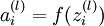这样我们就可以得到一种更简洁的表示法。这里我们将激活函数 $\textstyle f(\cdot)$ 扩展为用向量（分量的形式）来表示，即 $\textstyle f([z_1, z_2, z_3]) = [f(z_1), f(z_2), f(z_3)]$ ，那么，上面的等式可以更简洁地表示为：

$\begin{align} z^{(2)} &= W^{(1)} x + b^{(1)} \\ a^{(2)} &= f(z^{(2)}) \\ z^{(3)} &= W^{(2)} a^{(2)} + b^{(2)} \\ h_{W,b}(x) &= a^{(3)} = f(z^{(3)}) \end{align}$

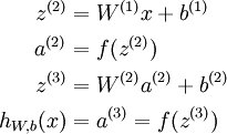
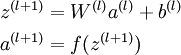
我们将上面的计算步骤叫作前向传播。回想一下，之前我们用 $\textstyle a^{(1)} = x$ 表示输入层的激活值，那么给定第 $\textstyle l$ 层的激活值 $\textstyle a^{(l)}$ 后，第 $\textstyle l+1$ 层的激活值 $\textstyle a^{(l+1)}$ 就可以按照下面步骤计算得到：

$\begin{align} z^{(l+1)} &= W^{(l)} a^{(l)} + b^{(l)} \\ a^{(l+1)} &= f(z^{(l+1)}) \end{align}$

将参数矩阵化，使用矩阵－向量运算方式，我们就可以利用线性代数的优势对神经网络进行快速求解。

目前为止，我们讨论了一种神经网络，我们也可以构建另一种结构的神经网络（这里结构指的是神经元之间的联接模式），也就是包含多个隐藏层的神经网络。最常见的一个例子是 $\textstyle n_l$ 层的神经网络，第 $\textstyle 1$ 层是输入层，第 $\textstyle n_l$ 层是输出层，中间的每个层 $\textstyle l$ 与层 $\textstyle l+1$ 紧密相联。这种模式下，要计算神经网络的输出结果，我们可以按照之前描述的等式，按部就班，进行前向传播，逐一计算第 $\textstyle L_2$ 层的所有激活值，然后是第 $\textstyle L_3$ 层的激活值，以此类推，直到第 $\textstyle L_{n_l}$ 层。这是一个前馈神经网络的例子，因为这种联接图没有闭环或回路。

神经网络也可以有多个输出单元。比如，下面的神经网络有两层隐藏层： $\textstyle L_2$ 及 $\textstyle L_3$ ，输出层 $\textstyle L_4$ 有两个输出单元。

要求解这样的神经网络，需要样本集 $\textstyle (x^{(i)}, y^{(i)})$ ，其中 $\textstyle y^{(i)} \in \Re^2$ 。如果你想预测的输出是多个的，那这种神经网络很适用。（比如，在医疗诊断应用中，患者的体征指标就可以作为向量的输入值，而不同的输出值 $\textstyle y_i$ 可以表示不同的疾病存在与否。）