
酒店评论的情感分析
一、情感分析
情感极性分析,即情感分类,对带有主观情感色彩的文本进行分析、归纳。情感极性分析主要有两种分类方法:基于情感知识的方法和基于机器学习的方法
基于情感知识的方法通过一些已有的情感词典计算文本的情感极性(正向或负向),其方法是统计文本中出现的正、负向情感词数目或情感词的情感值来判断文本情感类别
基于机器学习的方法利用机器学习算法训练已标注情感类别的训练数据集训练分类模型,再通过分类模型预测文本所属情感分类
本文采用机器学习方法实现对酒店评论数据的情感分类,旨在通过实践一步步了解、实现中文情感极性分析
下面详细介绍实战过程:
1)数据下载
a)停用词:
本文使用中科院计算所中文自然语言处理开放平台发布的中文停用词表,包含了1200多个停用词。下载地址:https://pan.baidu.com/s/1Eurf5unmYdjfmOl5ocRJDg 提取码:r8ee
b)正负向语料库:
文本从http://www.datatang.com/index.html下载“有关中文情感挖掘的酒店评论语料”作为训练集与测试集,该语料包含了4种语料子集,本文选用正负各1000的平衡语料(ChnSentiCorp_htl_ba_2000)作为数据集进行分析
数据集已经被我上传到百度文库:https://pan.baidu.com/s/1ABlob0A24tWS8lY5JICYBA 提取码:mavy,其中压缩文件包含了neg和pos文件夹,各含有1000个评论文本
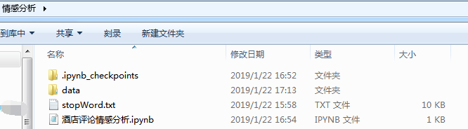
c)数据解压:
下载上面的数据后,在桌面新建情感分析文件夹,进入情感分析文件夹,新建data文件夹,然后将上面的压缩文件解压到data下面,并将stopWord.txt放于data平行目录
在情感分析文件夹下按住shift+鼠标右键,选择在此处新建dos窗口,然后输入jupyter notebook,新建酒店评论情感分析的脚本文件:
2)数据预处理
a)正负向语料预处理
为了方便之后的操作,需要把正向和负向评论分别规整到对应的一个txt文件中,即正向语料的集合文档(命名为2000_pos.txt)和负向语料的集合文档(命名为2000_neg.txt),这里注意encoding和errors参数的使用,否则会解码错误
这里的2000代表正负预料总共2000条数据
import logging
import os
import sys
import codecs

program = os.path.basename( sys.argv[0] )
logger = logging.getLogger( program )
logging.basicConfig( format='%(asctime)s: %(levelname)s: %(message)s' )
logging.root.setLevel( level=logging.INFO )

def getContent(fullname):
    f = codecs.open(fullname, 'r',  encoding="gbk", errors="ignore")
    lines = []
    for eachline in f:
        #eachline = eachline.decode('gbk','ignore').strip()
        eachline = eachline.strip()
        if eachline:#很多空行
            lines.append(eachline)
    f.close()
    #print(fullname, 'OK')
    return lines

inp = 'data/ChnSentiCorp_htl_ba_2000'
folders = ['neg', 'pos']
for foldername in folders:
    logger.info('running ' + foldername + ' files.')
    outp = '2000_' + foldername + '.txt'#输出文件
    output = codecs.open( os.path.join('data/ChnSentiCorp_htl_ba_2000', outp), 'w')
    i = 0

    rootdir = os.path.join(inp, foldername)
    for each_txt in os.listdir(rootdir):
        contents = getContent( os.path.join(rootdir, each_txt) )
        i = i + 1
        output.write(''.join(contents) + '\n' )

    output.close
    logger.info("Saved "+str(i)+" files.")
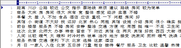
然后我们来看看合并后的文件(2000_pos.txt和2000_neg.txt)
b)中文文本分词,并去停顿词
采用结巴分词分别对正向语料和负向语料进行分词处理。在进行分词前,需要对文本进行去除数字、字母和特殊符号的处理,使用python自带的string和re模块可以实现
其中string模块用于处理字符串操作,re模块用于正则表达式处理。 具体实现代码如下所示:
import jieba
import os
import codecs
import re

def prepareData(sourceFile, targetFile):
    f =codecs.open(sourceFile, 'r', encoding='gbk')
    target = codecs.open(targetFile, 'w', encoding='gbk')
    print( 'open source file: '+ sourceFile )
    print( 'open target file: '+ targetFile )

    lineNum = 0
    for eachline in f:
        lineNum += 1
        print('---processing ', sourceFile, lineNum,' article---')
        eachline = clearTxt(eachline)
        #print( eachline )
        seg_line = sent2word(eachline)
        #print(seg_line)
        target.write(seg_line + '\n')
    print('---Well Done!!!---' * 4)
    f.close()
    target.close()


#文本清洗
def clearTxt(line):
    if line != '':
        line = line.strip()
        #去除文本中的英文和数字
        line = re.sub("[a-zA-Z0-9]","",line)

        #去除文本中的中文符号和英文符号
        line = re.sub("[\s+\.\!\/_,$%^*(+\"\';:“”.]+|[+——!,。??、~@#¥%……&*()]+", "", line)
        return line
    else:
        return 'Empyt Line'

#文本切割,并去除停顿词
def sent2word(line):

    segList = jieba.cut(line, cut_all=False)
    segSentence = ''
    for word in segList:
        if word != '\t' and ( word not in stopwords ):
            segSentence += ( word + " " )
    return segSentence.strip()

inp = 'data/ChnSentiCorp_htl_ba_2000'
stopwords = [ w.strip() for w in codecs.open('stopWord.txt', 'r', encoding='utf-8') ]

folders = ['neg', 'pos']
for folder in folders:
    sourceFile = '2000_{}.txt'.format(folder)
    targetFile = '2000_{}_cut.txt'.format(folder)
    prepareData( os.path.join(inp, sourceFile), os.path.join(inp,targetFile) )
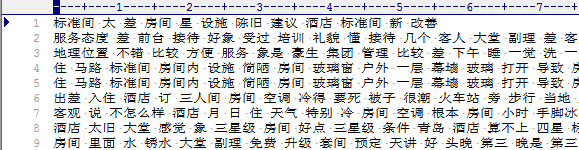
然后我们看一下分词结果(2000_pos_cut.txt和2000_neg_cut.txt):
c)获取特征词向量
根据以上步骤得到了正负向语料的特征词文本,而模型的输入必须是数值型数据,因此需要将每条由词语组合而成的语句转化为一个数值型向量。常见的转化算法有Bag of Words(BOW)、TF-IDF、Word2Vec
本文采用Word2Vec词向量模型将语料转换为词向量
由于特征词向量的抽取是基于已经训练好的词向量模型,而wiki中文语料是公认的大型中文语料,本文拟从wiki中文语料生成的词向量中抽取本文语料的特征词向量
Wiki中文语料的Word2vec模型训练在之前写过的一篇文章:“利用Python实现wiki中文语料的word2vec模型构建” 中做了详尽的描述,在此不赘述。即本文从文章最后得到的wiki.zh.text.vector中抽取特征词向量作为模型的输入
获取特征词向量的主要步骤如下:
1)读取模型词向量矩阵;
2)遍历语句中的每个词,从模型词向量矩阵中抽取当前词的数值向量,一条语句即可得到一个二维矩阵,行数为词的个数,列数为模型设定的维度;
3)根据得到的矩阵计算矩阵均值作为当前语句的特征词向量;
4)全部语句计算完成后,拼接语句类别代表的值,写入csv文件中
import os
import sys
import logging
import gensim
import codecs
import numpy as np
import pandas as pd

def getWordVecs(wordList, model):
    vecs = []
    for word in wordList:
        word = word.replace('\n', '')
        try:
            vecs.append(model[word])
        except KeyError:
            continue
    return np.array(vecs, dtype='float')


def buildVecs(filename, model):
    fileVecs = []
    with codecs.open(filename, 'r', encoding='gbk') as contents:
        for line in contents:
            logger.info('Start line: ' + line )
            wordList = line.strip().split(' ')#每一行去掉换行后分割
            vecs = getWordVecs(wordList, model)#vecs为嵌套列表,每个列表元素为每个分词的词向量
            if len(vecs) > 0:
                vecsArray = sum(np.array(vecs)) / len (vecs)
                fileVecs.append(vecsArray)
    return fileVecs

program = os.path.basename(sys.argv[0])
logger = logging.getLogger(program)
logging.basicConfig(format='%(asctime)s: %(levelname)s: %(message)s',level=logging.INFO)
logger.info("running %s" % ' '.join(sys.argv))

inp = 'data/ChnSentiCorp_htl_ba_2000/wiki.zh.text.vector'
model = gensim.models.KeyedVectors.load_word2vec_format(inp, binary=False)

posInput = buildVecs('data/ChnSentiCorp_htl_ba_2000/2000_pos_cut.txt', model)
negInput = buildVecs('data/ChnSentiCorp_htl_ba_2000/2000_neg_cut.txt', model)

Y = np.concatenate( ( np.ones(len(posInput)), np.zeros(len(negInput)) ) )

#这里也可以用np.concatenate将posInput和negInput进行合并
X = posInput[:]
for neg in negInput:
    X.append(neg)
X = np.array(X)
df_x = pd.DataFrame(X)
df_y = pd.DataFrame(Y)
data = pd.concat( [df_y, df_x], axis=1 )
data.to_csv('data/ChnSentiCorp_htl_ba_2000/2000_data.csv')
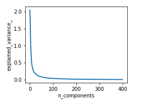
d)降维
Word2vec模型设定了400的维度进行训练,得到的词向量为400维,本文采用PCA算法对结果进行降维。具体实现代码如下所示(先看看我们需要降到多少维):
import sys
import numpy as np
import pandas as pd
import matplotlib.pyplot as plt
from sklearn.decomposition import PCA
from sklearn import svm
from sklearn import metrics

df = pd.read_csv('data/ChnSentiCorp_htl_ba_2000/2000_data.csv')
y = df.iloc[:, 1]#第一列是索引,第二列是标签
x = df.iloc[:, 2:]#第三列之后是400维的词向量

n_components = 400
pca = PCA(n_components=n_components)
pca.fit(x)

plt.figure(1, figsize=(4,3) )
plt.clf()
plt.axes( [.2, .2, .7, .7] )
plt.plot( pca.explained_variance_, linewidth=2)
plt.axis('tight')
plt.xlabel('n_components')
plt.ylabel('explained_variance_')
plt.show()
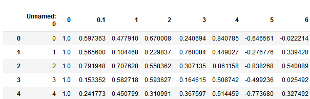
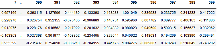
代码示例结果,展示df前5行:
e)分类模型构建
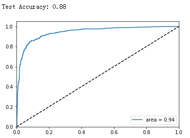
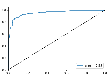
支持向量机(SVM)是一种有监督的机器学习模型。本文首先采用经典的机器学习算法SVM作为分类器算法,通过计算测试集的预测精度和ROC曲线来验证分类器的有效性,一般来说ROC曲线的面积(AUC)越大模型的表现越好
##根据图形取100维
import warnings
warnings.filterwarnings('ignore')
x_pca = PCA(n_components = 100).fit_transform(x)

# SVM (RBF)
# using training data with 100 dimensions

clf = svm.SVC(C = 2, probability = True)
clf.fit(x_pca,y)

print ('Test Accuracy: %.2f'% clf.score(x_pca,y))
#Create ROC curve
pred_probas = clf.predict_proba(x_pca)[:,1] #score

fpr,tpr,_ = metrics.roc_curve(y, pred_probas)
roc_auc = metrics.auc(fpr,tpr)
plt.plot(fpr, tpr, label = 'area = %.2f' % roc_auc)
plt.plot([0, 1], [0, 1], 'k--')
plt.xlim([0.0, 1.0])
plt.ylim([0.0, 1.05])
plt.legend(loc = 'lower right')
plt.show()
运行代码,得到Test Accuracy: 0.88,即本次实验测试集的预测准确率为88%,ROC曲线如下图所示:
二、模型构建,训练
上面的SVM模型并未对数据集进行训练和测试的拆分,我们下面将数据集进行拆分,test_size设置为0.25,我们先看看AUC判断标准
AUC的一般判断标准
0.5 - 0.7:效果较低,但用于预测股票已经很不错了
0.7 - 0.85:效果一般
0.85 - 0.95:效果很好
0.95 - 1:效果非常好,但一般不太可能
a)逻辑回归
from sklearn.model_selection import train_test_split
import numpy as np
from sklearn.linear_model import LogisticRegression
from sklearn.metrics import accuracy_score
from sklearn.metrics import classification_report
from sklearn.model_selection import GridSearchCV
from sklearn import metrics
def show_roc(model, X, y):
#Create ROC curve
pred_probas = model.predict_proba(X)[:,1]#score
fpr,tpr,_ = metrics.roc_curve(y, pred_probas)
roc_auc = metrics.auc(fpr,tpr)
plt.plot(fpr, tpr, label = 'area = %.2f' % roc_auc)
plt.plot([0, 1], [0, 1], 'k--')
plt.xlim([0.0, 1.0])
plt.ylim([0.0, 1.05])
plt.legend(loc = 'lower right')
plt.show()
X_train, X_test, y_train, y_test = train_test_split( x_pca, y, test_size=0.25, random_state=0)
param_grid = {'C': [0.01,0.1, 1, 10, 100, 1000,],'penalty': [ 'l1', 'l2']}
grid_search = GridSearchCV(LogisticRegression(), param_grid, cv=10)
grid_search.fit( X_train,y_train )
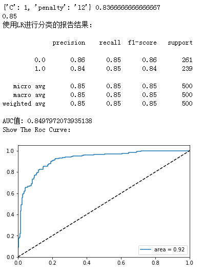
print( grid_search.best_params_, grid_search.best_score_ )
#预测拆分的test
LR = LogisticRegression( C=grid_search.best_params_['C'], penalty=grid_search.best_params_['penalty'] )
LR.fit( X_train,y_train )
lr_y_predict = LR.predict(X_test)
print(accuracy_score(y_test, lr_y_predict))
print('使用LR进行分类的报告结果:\n')
print(classification_report(y_test, lr_y_predict))
print( "AUC值:",roc_auc_score( y_test, lr_y_predict ) )
print('Show The Roc Curve:')
show_roc(LR, X_test, y_test)
代码示例结果:
这里我们用网格搜索进行了参数的调整,但有个小疑问,为何roc_auc_score求出的AUC与图上的area不一致呢?
b)Xgboost
import xgboost as xgb
from xgboost import XGBClassifier
from sklearn.metrics import accuracy_score
from sklearn.model_selection import GridSearchCV
from sklearn.metrics import roc_auc_score

def modelfit(alg, dtrain_x, dtrain_y, useTrainCV=True, cv_flods=5, early_stopping_rounds=50):
    """
    :param alg: 初始模型
    :param dtrain_x:训练数据X
    :param dtrain_y:训练数据y(label)
    :param useTrainCV: 是否使用cv函数来确定最佳n_estimators
    :param cv_flods:交叉验证的cv数
    :param early_stopping_rounds:在该数迭代次数之前,eval_metric都没有提升的话则停止
    """
    if useTrainCV:
        xgb_param = alg.get_xgb_params()
        xgtrain = xgb.DMatrix(dtrain_x, dtrain_y)
        print(alg.get_params()['n_estimators'])

        cv_result = xgb.cv( xgb_param, xgtrain, num_boost_round = alg.get_params()['n_estimators'],
                        nfold=cv_flods, metrics = 'auc', early_stopping_rounds = early_stopping_rounds )

        print('useTrainCV\n',cv_result)
        print('Total estimators:',cv_result.shape[0])
        alg.set_params(n_estimators=cv_result.shape[0])

    # train data
    alg.fit(dtrain_x, dtrain_y, eval_metric='auc')

    #predict train data
    train_y_pre = alg.predict(dtrain_x)
    print ("\nModel Report")
    print ("Accuracy : %.4g" % accuracy_score( dtrain_y, train_y_pre) )

    return cv_result.shape[0]


#XGBoost调参
def xgboost_change_param(train_X, train_y):

    print('######Xgboost调参######')
    print('\n step1 确定学习速率和迭代次数n_estimators')

    xgb1 = XGBClassifier(learning_rate=0.1, booster='gbtree', n_estimators=1000,
                         max_depth=4, min_child_weight=1,
                         gamma=0, subsample=0.8, colsample_bytree=0.8,
                         objective='binary:logistic',scale_pos_weight=1, seed=10)

    #useTrainCV=True时,最佳n_estimators=23, learning_rate=0.1
    NEstimators = modelfit(xgb1, train_X, train_y, early_stopping_rounds=45)

    print('\n step2 调试参数min_child_weight以及max_depth')
    param_test1 = { 'max_depth' : range(3, 8, 1), 'min_child_weight' : range(1, 6, 2) }

    #GridSearchCV()中的estimator参数所使用的分类器
    #并且传入除需要确定最佳的参数之外的其他参数
    #每一个分类器都需要一个scoring参数,或者score方法
    gsearch1 = GridSearchCV( estimator=XGBClassifier( learning_rate=0.1,n_estimators=NEstimators,
                                                     gamma=0,subsample=0.8,colsample_bytree=0.8,
                                                     objective='binary:logistic',scale_pos_weight=1,seed=10 ),
                            param_grid=param_test1,scoring='roc_auc', cv=5)

    gsearch1.fit(train_X,train_y)
    #最佳max_depth = 4 min_child_weight=1
    print(gsearch1.best_params_, gsearch1.best_score_)
    MCW = gsearch1.best_params_['min_child_weight']
    MD = gsearch1.best_params_['max_depth']

    print('\n step3 gamma参数调优')
    param_test2 = { 'gamma': [i/10.0 for i in range(0,5)] }

    gsearch2 = GridSearchCV( estimator=XGBClassifier(learning_rate=0.1,n_estimators=NEstimators,
                                                    max_depth=MD, min_child_weight=MCW,
                                                    subsample=0.8,colsample_bytree=0.8,
                                                    objective='binary:logistic',scale_pos_weight=1,seed=10),
                            param_grid=param_test2,scoring='roc_auc',cv=5 )

    gsearch2.fit(train_X, train_y)
    #最佳 gamma = 0.0
    print(gsearch2.best_params_, gsearch2.best_score_)
    GA = gsearch2.best_params_['gamma']

    print('\n step4 调整subsample 和 colsample_bytrees参数')
    param_test3 = { 'subsample': [i/10.0 for i in range(6,10)],
                   'colsample_bytree': [i/10.0 for i in range(6,10)] }

    gsearch3 = GridSearchCV( estimator=XGBClassifier(learning_rate=0.1,n_estimators=NEstimators,
                                                     max_depth=MD,min_child_weight=MCW,gamma=GA,
                                                     objective='binary:logistic',scale_pos_weight=1,seed=10),
                            param_grid=param_test3,scoring='roc_auc',cv=5 )

    gsearch3.fit(train_X, train_y)
    #最佳'subsample': 0.8, 'colsample_bytree': 0.8
    print(gsearch3.best_params_, gsearch3.best_score_)
    SS = gsearch3.best_params_['subsample']
    CB = gsearch3.best_params_['colsample_bytree']

    print('\nstep5 正则化参数调优')
    param_test4= { 'reg_alpha':[1e-5, 1e-2, 0.1, 1, 100] }
    gsearch4= GridSearchCV(estimator=XGBClassifier(learning_rate=0.1,n_estimators=NEstimators,
                                                   max_depth=MD,min_child_weight=MCW,gamma=GA,
                                                   subsample=SS,colsample_bytree=CB,
                                                   objective='binary:logistic',
                                                   scale_pos_weight=1,seed=10),
                           param_grid=param_test4,scoring='roc_auc',cv=5 )
    gsearch4.fit(train_X, train_y)
    #reg_alpha:1e-5
    print(gsearch4.best_params_, gsearch4.best_score_)
    RA = gsearch4.best_params_['reg_alpha']

    param_test5 ={ 'reg_lambda':[1e-5, 1e-2, 0.1, 1, 100] }
    gsearch5= GridSearchCV(estimator=XGBClassifier(learning_rate=0.1,n_estimators=NEstimators,
                                                   max_depth=MD,min_child_weight=MCW,gamma=GA,
                                                   subsample=SS,colsample_bytree=CB,
                                                   objective='binary:logistic',reg_alpha=RA,
                                                   scale_pos_weight=1,seed=10),
                           param_grid=param_test5,scoring='roc_auc',cv=5)

    gsearch5.fit(train_X, train_y)
    #reg_lambda:1
    print(gsearch5.best_params_, gsearch5.best_score_)
    RL = gsearch5.best_params_['reg_lambda']

    return NEstimators, MD, MCW, GA, SS, CB, RA, RL

# XGBoost调参
X_train = np.array(X_train)
#返回最佳参数
NEstimators, MD, MCW, GA, SS, CB, RA, RL = xgboost_change_param(X_train, y_train)

#parameters at last
print( '\nNow we use the best parasms to fit and predict:\n' )
print( 'n_estimators = ', NEstimators)
print( 'max_depth = ', MD)
print( 'min_child_weight = ', MCW)
print( 'gamma = ', GA)
print( 'subsample = ', SS)
print( 'colsample_bytree = ', CB)
print( 'reg_alpha = ', RA)
print( 'reg_lambda = ', RL)
xgb1 = XGBClassifier(learning_rate=0.1,n_estimators=NEstimators,max_depth=MD,min_child_weight=MCW,
                     gamma=GA,subsample=SS,colsample_bytree=CB,objective='binary:logistic',reg_alpha=RA,reg_lambda=RL,
                     scale_pos_weight=1,seed=10)
xgb1.fit(X_train, y_train)
xgb_test_pred = xgb1.predict( np.array(X_test) )
print ("The xgboost model Accuracy : %.4g" % accuracy_score(y_pred=xgb_test_pred, y_true=y_test))
print('使用Xgboost进行分类的报告结果:\n')
print( "AUC值:",roc_auc_score( y_test, xgb_test_pred ) )
print( classification_report(y_test, xgb_test_pred) )
print('Show The Roc Curve:')
show_roc(xgb1, X_test, y_test)
代码示例结果:
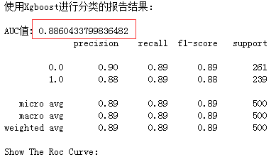
从结果上看,Xgboost比LR效果强一些,感兴趣的读者可以使用神经网络来进行情感分析

 浙公网安备 33010602011771号