增长模型:R 语言复现
-
课程开始时,鉴于电子商务专业的同学编程能力很强,教师承诺过会给一个关于增长模型的代码复现例子。
-
Here we go!
MRW 1992
-
数据和模型均来自论文, “A Contribution to the Empirics of Economic Growth”
- Greg Mankiw, David Romer and David Weil (QJE, 1992)
-
索洛模型:储蓄率和人口增长率决定了稳态时的人均收入
-
问:现实中,储蓄率和人口增长率低的国家,人均 GDP 会更高么?
-
MRW: 对,但不完全对
-
储蓄率和人口增长率只能解释不同国家质检约 50% 的收入差距
-
如果加入人力资本,可以解释 80% 的收入差距
模型设定
\[Y(t) = K(t)^\alpha [A(t) L(t)]^{1-\alpha} \; \text{where} \; 0 < \alpha < 1
\]
\[L(t) = L(0) e^{nt}
\]
\[A(t) = A(0) e^{gt}
\]
\[\dot{k}(t) = sk(t)^\alpha - (n+g+\delta)k(t)
\]
\[k^* = [\frac{s}{n+g+\delta}]^{\frac{1}{1-a}}
\]
- 其中 \(\alpha = 2/3\)
Exploratory data analysis
library(AER)
library(dplyr)
library(skimr)
library(moderndive)
data("GrowthDJ")

skim(GrowthDJ)
── Data Summary ────────────────────────
                           Values
Name                       GrowthDJ
Number of rows             121
Number of columns          10
_______________________
Column type frequency:
  factor                   3
  numeric                  7
________________________
Group variables            None

── Variable type: factor ──────────────────────────────────────────────────────────────────────────
  skim_variable n_missing complete_rate ordered n_unique top_counts
1 oil                   0             1 FALSE          2 no: 98, yes: 23
2 inter                 0             1 FALSE          2 yes: 75, no: 46
3 oecd                  0             1 FALSE          2 no: 99, yes: 22

── Variable type: numeric ─────────────────────────────────────────────────────────────────────────
  skim_variable n_missing complete_rate    mean       sd    p0    p25     p50     p75    p100 hist
1 gdp60                 5         0.959 3682.   7493.    383    973.  1962    4274.   77881   ▇▁▁▁▁
2 gdp85                13         0.893 5683.   5689.    412   1209.  3484.   7719.   25635   ▇▂▂▁▁
3 gdpgrowth             4         0.967    4.09    1.89   -0.9    2.8    3.9     5.3      9.2 ▁▅▇▃▁
4 popgrowth            14         0.884    2.28    0.999   0.3    1.7    2.4     2.9      6.8 ▃▇▃▁▁
5 invest                0         1       18.2     7.85    4.1   12     17.7    24.1     36.9 ▅▇▇▅▂
6 school                3         0.975    5.53    3.53    0.4    2.4    4.95    8.17    12.1 ▇▆▅▅▅
7 literacy60           18         0.851   48.2    35.4     1     15     39      83.5    100   ▇▃▂▃▆
Estimation
-
参数校准:\(g + \delta = 0.5\)
-
下面以 MRW 中数据中的样本 1 为例进行估计
nonoil <- subset(GrowthDJ, oil == "no")
inter <- subset(GrowthDJ, inter == "yes")
oecd <- subset(GrowthDJ, oecd == "yes")

mrw1 <- lm(log(gdp85) ~ log(invest/100) + log((popgrowth/100) + 0.05), data = nonoil)
mrw2 <- lm(log(gdp85) ~ log(invest/100) + log((popgrowth/100) + 0.05), data = inter)
mrw3 <- lm(log(gdp85) ~ log(invest/100) + log((popgrowth/100) + 0.05), data = oecd)

summary(mrw1)
Residuals:
     Min       1Q   Median       3Q      Max
-1.79144 -0.39367  0.04124  0.43368  1.58046

Coefficients:
                            Estimate Std. Error t value Pr(>|t|)
(Intercept)                   5.4299     1.5839   3.428 0.000900 ***
log(invest/100)               1.4240     0.1431   9.951  < 2e-16 ***
log((popgrowth/100) + 0.05)  -1.9898     0.5634  -3.532 0.000639 ***
---
Signif. codes:  0 ‘***’ 0.001 ‘**’ 0.01 ‘*’ 0.05 ‘.’ 0.1 ‘ ’ 1

Residual standard error: 0.6891 on 95 degrees of freedom
Multiple R-squared:  0.6009,	Adjusted R-squared:  0.5925
F-statistic: 71.51 on 2 and 95 DF,  p-value: < 2.2e-16
Restricted regression
- Restriction: \(\ln (s)\) 与 \(\ln(g+n+\delta)\) 的和为0
mrw4 <- lm(log(gdp85) ~ I(log(invest/100) - log((popgrowth/100) + 0.05)), data = nonoil)
mrw5 <- lm(log(gdp85) ~ I(log(invest/100) - log((popgrowth/100) + 0.05)), data = inter)
mrw6 <- lm(log(gdp85) ~ I(log(invest/100) - log((popgrowth/100) + 0.05)), data = oecd)

summary(mrw4)
Residuals:
     Min       1Q   Median       3Q      Max
-1.87388 -0.43133  0.03757  0.51698  1.49645

Coefficients:
                                                 Estimate Std. Error t value Pr(>|t|)
(Intercept)                                        6.8724     0.1206   56.99   <2e-16 ***
I(log(invest/100) - log((popgrowth/100) + 0.05))   1.4880     0.1247   11.93   <2e-16 ***
---
Signif. codes:  0 ‘***’ 0.001 ‘**’ 0.01 ‘*’ 0.05 ‘.’ 0.1 ‘ ’ 1

Residual standard error: 0.6885 on 96 degrees of freedom
Multiple R-squared:  0.5974,	Adjusted R-squared:  0.5932
F-statistic: 142.4 on 1 and 96 DF,  p-value: < 2.2e-16
-
运算结果表明,\((N+g+\delta)\) 的系数显著为负,而储蓄 \(s\) 的系数显著为正
- 这和索洛模型的预测一致
-
但是,restricted regression 中计算得到的 \(\alpha= 0.6\), 和实际不符
考虑加入人力资本的有效劳动人口
- 衡量人力资本:使用不同时间段的“劳动人口中完成中学教育的比例”作为代理变量
- 从 \(R^2\) 可以看出,加入人力资本后的索洛模型,可以解释不同国家之间 80% 的收入差距
- 同时,\(\alpha\) 的取值也接近 1/3. 这和实际数据一致
- 因此,加入人力资本后的索洛模型,能更好地解释不通国家之间的收入差距
mrw7 <- lm(log(gdp85) ~ log(invest/100) + log((popgrowth/100) + 0.05) + log(school/100), data = nonoil)
mrw8 <- lm(log(gdp85) ~ log(invest/100) + log((popgrowth/100) + 0.05) + log(school/100), data = inter)
mrw9 <- lm(log(gdp85) ~ log(invest/100) + log((popgrowth/100) + 0.05) + log(school/100), data = oecd)
mrw10 <- lm(log(gdp85) ~ I(log(invest/100) - log((popgrowth/100) + 0.05)) + I(log(school/100) - log((popgrowth/100) + 0.05)), data = nonoil)
mrw11 <- lm(log(gdp85) ~ I(log(invest/100) - log((popgrowth/100) + 0.05)) + I(log(school/100) - log((popgrowth/100) + 0.05)), data = inter)
mrw12 <- lm(log(gdp85) ~ I(log(invest/100) - log((popgrowth/100) + 0.05)) + I(log(school/100) - log((popgrowth/100) + 0.05)), data = oecd)
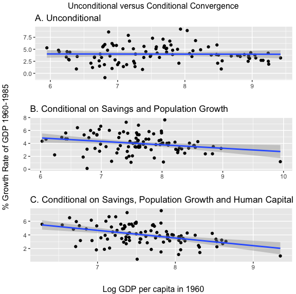
收敛和条件收敛
- 索洛模型的另一个主要预测,是有类似条件的国家,稳态时的人均 GDP 会收敛 (conditional convergence)
- 此外,它还定量说明了收敛的速度
- 我们用 1960--1985 年之间不同国家的相关数据,对这个预测进行检验
converge1 <- lm(I(log(gdp85)-log(gdp60)) ~ log(gdp60), data = nonoil)

summary(converge1)

Residuals:
     Min       1Q   Median       3Q      Max
-1.09784 -0.27467 -0.02826  0.25975  1.17747

Coefficients:
            Estimate Std. Error t value Pr(>|t|)
(Intercept) -0.26658    0.37960  -0.702   0.4842
log(gdp60)   0.09431    0.04962   1.901   0.0603 .
---
Signif. codes:  0 ‘***’ 0.001 ‘**’ 0.01 ‘*’ 0.05 ‘.’ 0.1 ‘ ’ 1

Residual standard error: 0.4405 on 96 degrees of freedom
Multiple R-squared:  0.03627,	Adjusted R-squared:  0.02623
F-statistic: 3.613 on 1 and 96 DF,  p-value: 0.06033

converge4 <- lm(I(log(gdp85)-log(gdp60)) ~ log(gdp60) + log(invest/100) + log(popgrowth/100 + 0.05), data = nonoil)

summary(converge4)
Residuals:
     Min       1Q   Median       3Q      Max
-1.07648 -0.15215  0.01185  0.19595  0.96056

Coefficients:
                          Estimate Std. Error t value Pr(>|t|)
(Intercept)                1.91938    0.83367   2.302  0.02352 *
log(gdp60)                -0.14090    0.05202  -2.709  0.00803 **
log(invest/100)            0.64724    0.08670   7.465 4.16e-11 ***
log(popgrowth/100 + 0.05) -0.30235    0.30438  -0.993  0.32311
---
Signif. codes:  0 ‘***’ 0.001 ‘**’ 0.01 ‘*’ 0.05 ‘.’ 0.1 ‘ ’ 1

Residual standard error: 0.3507 on 94 degrees of freedom
Multiple R-squared:  0.4019,	Adjusted R-squared:  0.3828
F-statistic: 21.05 on 3 and 94 DF,  p-value: 1.622e-10
converge7 <- lm(I(log(gdp85)-log(gdp60)) ~ log(gdp60) + log(invest/100) + log(popgrowth/100 + 0.05) + log(school/100), data = nonoil)

summary(converge7)
Residuals:
     Min       1Q   Median       3Q      Max
-0.91041 -0.17599  0.01789  0.18439  0.93846

Coefficients:
                          Estimate Std. Error t value Pr(>|t|)
(Intercept)                3.02152    0.82748   3.651 0.000431 ***
log(gdp60)                -0.28837    0.06158  -4.683 9.62e-06 ***
log(invest/100)            0.52374    0.08687   6.029 3.30e-08 ***
log(popgrowth/100 + 0.05) -0.50566    0.28861  -1.752 0.083061 .
log(school/100)            0.23112    0.05946   3.887 0.000190 ***
---
Signif. codes:  0 ‘***’ 0.001 ‘**’ 0.01 ‘*’ 0.05 ‘.’ 0.1 ‘ ’ 1

Residual standard error: 0.327 on 93 degrees of freedom
Multiple R-squared:  0.4855,	Adjusted R-squared:  0.4633
F-statistic: 21.94 on 4 and 93 DF,  p-value: 8.987e-13
回归结果:
-
不存在绝对收敛
-
控制储蓄率和人口增长后,存在条件收敛的趋势
-
进一步控制人力资本变量后,条件收敛的趋势非常明显
收敛图示
library(ggplot2)
library(gridExtra)

controlx1 <- lm(log(gdp60) ~ log(invest/100) + log(popgrowth/100 + 0.05), data = nonoil)
controlx1res <- residuals(controlx1)


controly1 <- lm(gdpgrowth ~ log(invest/100) + log(popgrowth/100 + 0.05), data = nonoil)
controly1res <- residuals(controly1)


controlx2 <- lm(log(gdp60) ~ log(invest/100) + log(popgrowth/100 + 0.05) + log(school/100), data = nonoil)
controlx2res <- residuals(controlx2)

controly2 <- lm(gdpgrowth ~ log(invest/100) + log(popgrowth/100 + 0.05) + log(school/100), data = nonoil)
controly2res <- residuals(controly2)


p1 <- ggplot(data = nonoil, mapping = aes(x=log(gdp60), y=gdpgrowth)) + geom_point() + geom_smooth(method = "lm") + labs(title = "A. Unconditional", x = "", y="")
p2 <- ggplot(data = nonoil, mapping = aes(x=(mean(log(gdp60))+controlx1res), y=(mean(gdpgrowth)+controly1res))) + geom_point() + geom_smooth(method = "lm") + labs(title = "B. Conditional on Savings and Population Growth", x = "", y="")
p3 <- ggplot(data = nonoil, mapping = aes(x=(mean(log(gdp60))+controlx2res), y=(mean(gdpgrowth)+controly2res))) + geom_point() + geom_smooth(method = "lm") + labs(title = "C. Conditional on Savings, Population Growth and Human Capital", x = "", y="")

grid.arrange(p1, p2, p3, ncol=1, top = "Unconditional versus Conditional Convergence", left = "% Growth Rate of GDP 1960-1985", bottom = "Log GDP per capita in 1960")
posted on 2021-06-18 20:19 Albert_Lei 阅读(429) 评论(0) 收藏 举报

 浙公网安备 33010602011771号