菜鸟之路——机器学习之SVM分类器学习理解以及Python实现

SVM分类器里面的东西好多呀，碾压前两个。怪不得称之为深度学习出现之前表现最好的算法。

今天学到的也应该只是冰山一角，懂了SVM的一些原理。还得继续深入学习理解呢。

一些关键词：

超平面（hyper plane）SVM的目标就是找到一个超平面把两类数据分开。使边际（margin）最大。如果把超平面定义为w*x+b=0.那么超平面距离任意一个支持向量的距离就是1/||w||。（||w||是w的范数，也就是√w*w’）

SVM就是解决

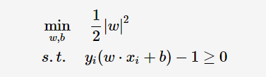
这个优化问题。再经过拉格朗日公式和KKT条件等数学运算求解得到一个d（X^T）=∑yi*a_i X^T +b0。y_i是类别标记，X_i是支持向量点。X^T是待预测实例的转置。a_i，b₀是求解出的固定值。根据d（X^T）的正负判断分类。

简单来说就是这样的。下面写一个简单的程序

线性可分

 1 import numpy as np
 2 import pylab as pl   #画图用
 3 from sklearn import svm
 4 
 5 #随机生成两组二位数据
 6 np.random.seed(0)#使每次产生随机数不变
 7 X = np.r_[np.random.randn(20,2)-[2,2],np.random.randn(20,2)+[2,2]]#注意这里np.r_[],而不是np.r_（）我都打错了，会报错TypeError: 'RClass' object is not callable
 8 #np.r_是按列连接两个矩阵，就是把两矩阵上下相加，要求列数相等，np.c_是按行连接两个矩阵，就是把两矩阵左右相加，要求行数相等
 9 
10 Y = [0] * 20+[1] * 20#Python原来可以这么简单的创建重复的列表呀
11 
12 clf=svm.SVC(kernel='linear')
13 clf.fit(X,Y)
14 
15 w=clf.coef_[0]
16 a=-w[0]/w[1]
17 xx=np.linspace(-5,5)#产生-5到5的线性连续值，间隔为1
18 yy=a*xx-(clf.intercept_[0])/w[1]  #clf.intercept_[0]是w3.即为公式a1*x1+a2*x2+w3中的w3。(clf.intercept_[0])/w[1]即为直线的截距
19 
20 #得出支持向量的方程
21 b=clf.support_vectors_[0]
22 yy_down=a*xx+(b[1]-a*b[0])#(b[1]-a*b[0])就是简单的算截距
23 b=clf.support_vectors_[-1]
24 yy_up=a*xx+(b[1]-a*b[0])
25 
26 print("w:",w) #打印出权重系数
27 print("a:",a) #打印出斜率
28 print("suport_vectors_:",clf.support_vectors_)#打印出支持向量
29 print("clf.coef_:",clf.coef_)                  #打印出权重系数，还是w
30 
31 
32 #这个就是画出来而已。很简单，也不太常用，都用matplotlib去了。不多说了
33 pl.plot(xx,yy,'k-')
34 pl.plot(xx,yy_down,'k--')
35 pl.plot(xx,yy_up,'k--')
36 
37 pl.scatter(clf.support_vectors_[:,0],clf.support_vectors_[:,0],s=80,facecolors='none')
38 pl.scatter(X[:,0],X[:,1],c=Y,cmap=pl.cm.Paired)
39 
40 pl.axis('tight')
41 pl.show()

小知识点：

np.r_是按列连接两个矩阵，就是把两矩阵上下相加，要求列数相等，np.c_是按行连接两个矩阵，就是把两矩阵左右相加，要求行数相等

运行之后就是

w: [0.90230696 0.64821811]
a: -1.391980476255765
suport_vectors_: [[-1.02126202 0.2408932 ]
[-0.46722079 -0.53064123]
[ 0.95144703 0.57998206]]
clf.coef_: [[0.90230696 0.64821811]]

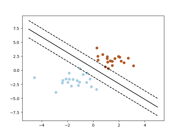
实线就是传说中的超平面，虚线就是支持向量所在的直线。

线性不可分

接下来就是线性不可分的情况啦。

顾名思义就是一根直线划分不出来两个类。

这样的话就用一个非线性的映射转化到一个更高维度的空间中。很好理解。比如一维的[-1,0,1]三个点，0是一类，（-1,1）是另一类。一根直线不可能分开，那就用一个y=x²转化为了[(-1,1),(0,0),(1,1)]这样的话就能用一根直线分开啦，比如，y=0.5这个直线。这不画图了，可以自行画图理解一下，高维亦然。

但是吧转化到高维可以分类了，然而又不便于计算了。维度越高，内积算的越慢，就令K（x_i，y_i）=φ（x_i）·φ（y_i）=x1*y1+x2*y2+......+xn*yn。这里的φ（x）就是上面说的映射。

核函数就简化了算内积的数量。让程序运行更快。将映射后的高维空间内积转换成低维空间的函数。

常用的核函数：

线性核函数（Linear Kernel）： $K (x, z) = x ∙ z$

多项式核函数： $K (x, z) = （ γ x ∙ z + r)^{d}$ $γ, r, d$

　　　高斯核函数（Gaussian Kernel）：K(x,z)=exp(−γ||x−z||2)，也称为径向基核函数（Radial Basis Function,RBF），它是非线性分类SVM最主流的核函数。libsvm默认的核函数就是它。γ大于0，需要自己调参定义。

Sigmoid核函数（Sigmoid Kernel）： $K (x, z) = t a n h （ γ x ∙ z + r)$ γ,r

对于多类的分类问题。一般都对于每个类，有以下当前类和其他类的二类分类器。

下面是一个人脸识别的程序。

 1 #from __future__ import print_function #__future__模块，把下一个新版本的特性导入到当前版本，于是我们就可以在当前版本中测试一些新版本的特性
 2                                         #我的Python版本是3.6.4.所以不需要这个
 3 
 4 from time import time   #对程序运行时间计时用的
 5 import logging           #打印程序进展日志用的
 6 import matplotlib.pyplot as plt  #绘图用的
 7 
 8 from sklearn.model_selection import train_test_split
 9 from sklearn.datasets import fetch_lfw_people
10 from sklearn.model_selection import GridSearchCV
11 from sklearn.metrics import classification_report
12 from sklearn.metrics import confusion_matrix
13 from sklearn.decomposition import PCA
14 from sklearn.svm import SVC
15 
16 logging.basicConfig(level=logging.INFO,format='%(asctime)s %(message)s')
17 lfw_people=fetch_lfw_people(min_faces_per_person=70,resize=0.4)  #名人的人脸数据集、
18 
19 n_samples,h,w=lfw_people.images.shape  #多少个实例，h,w高度，宽度值
20 
21 X=lfw_people.data   #特征向量矩阵
22 n_feature=X.shape[1]#每个人有多少个特征值
23 
24 Y=lfw_people.target
25 target_names=lfw_people.target_names
26 n_classes=target_names.shape[0]     #多少类
27 print("Total dataset size")
28 print("n_samples:",n_samples)
29 print("n_feature:",n_feature)
30 print("n_classes:",n_classes)
31 
32 X_train,X_test,Y_train,Y_test=train_test_split(X,Y,test_size=0.25)  #选取0.25的测试集
33 
34 #降维
35 n_components=150  #PCA算法中所要保留的主成分个数n，也即保留下来的特征个数n
36 print("Extracting the top %d eigenfaces from %d faces" % (n_components,X_train.shape[0]))
37 t0=time()
38 pca=PCA(svd_solver='randomized',n_components=n_components,whiten=True).fit(X_train)#训练一个pca模型
39 
40 print("Train PCA in %0.3fs" % (time()-t0))
41 
42 eigenfaces  = pca.components_.reshape((n_components,h,w))  #提取出来特征值之后的矩阵
43 
44 print("Prijecting the input data on the eigenfaces orthonarmal basis")
45 t0=time()
46 X_train_pca = pca.transform(X_train)     #将训练集与测试集降维
47 X_test_pca = pca.transform(X_test)
48 print("Done PCA in %0.3fs" % (time()-t0))
49 
50 
51 #终于到SVM训练了
52 print("Fiting the classifier to the training set")
53 t0=time()
54 param_grid ={'C':[1e3,5e3,1e4,5e4,1e5],#C是对错误的惩罚
55              'gamma':[0.0001,0.0005,0.001,0.005,0.01,0.1],}#gamma核函数里多少个特征点会被使用}#对参数尝试不同的值
56 clf = GridSearchCV(SVC(kernel='rbf'),param_grid)
57 clf=clf.fit(X_train_pca,Y_train)
58 print("Done Fiting in %0.3fs" % (time()-t0))
59 
60 print("Best estimotor found by grid search:")
61 print(clf.best_estimator_)
62 
63 print("Predicting people's names on the test set")
64 t0=time()
65 Y_pred = clf.predict(X_test_pca)
66 print("done Predicting in %0.3fs" % (time()-t0))
67 
68 print(classification_report(Y_test,Y_pred,target_names=target_names)) #生成一个小报告呀
69 print(confusion_matrix(Y_test,Y_pred,labels=range(n_classes)))#这个也是，生成的矩阵的意思是有多少个被分为此类。
70 
71 
72 #把分类完的图画出来12个。
73 
74 #这个函数就是画图的
75 def plot_gallery(images,titles,h,w,n_row=3,n_col=4):
76     plt.figure(figsize=(1.8*n_col,2.4*n_row))
77     plt.subplots_adjust(bottom=0,left=.01,right=.99,top=.90,hspace=.35)
78     for i in range(n_row*n_col):
79         plt.subplot(n_row,n_col,i+1)
80         plt.imshow(images[i].reshape((h,w)),cmap=plt.cm.gray)
81         plt.title(titles[i],size=12)
82         plt.xticks(())
83         plt.yticks(())
84         
85 #这个函数是生成一个固定格式的字符串的
86 def title(y_pred,y_test,target_names,i):
87     pred_name=target_names[y_pred[i]].rsplit(' ',1)[-1]
88     true_name = target_names[y_test[i]].rsplit(' ', 1)[-1]
89     return "predicted: %s\n true: %s" %(pred_name,true_name)
90 
91 predicted_titles=[title(Y_pred,Y_test,target_names,i) for i in range(Y_pred.shape[0])] #这个for循环的用法很简介
92 
93 plot_gallery(X_test,predicted_titles,h,w)
94 
95 eigenfaces_titles=["eigenface %d " % i for i in range(eigenfaces.shape[0])]
96 plot_gallery(eigenfaces,eigenfaces_titles,h,w)
97 
98 plt.show()

运行结果为

Total dataset size
n_samples: 1288
n_feature: 1850
n_classes: 7
Extracting the top 150 eigenfaces from 966 faces
Train PCA in 0.440s
Prijecting the input data on the eigenfaces orthonarmal basis
Done PCA in 0.019s
Fiting the classifier to the training set
Done Fiting in 52.087s
Best estimotor found by grid search:
SVC(C=1000.0, cache_size=200, class_weight=None, coef0=0.0,
decision_function_shape='ovr', degree=3, gamma=0.001, kernel='rbf',
max_iter=-1, probability=False, random_state=None, shrinking=True,
tol=0.001, verbose=False)
Predicting people's names on the test set
done Predicting in 0.147s
precision recall f1-score support

Ariel Sharon 0.75 0.80 0.77 15
Colin Powell 0.81 0.86 0.84 59
Donald Rumsfeld 0.86 0.81 0.83 37
George W Bush 0.90 0.90 0.90 134
Gerhard Schroeder 0.77 0.82 0.79 28
Hugo Chavez 0.92 0.86 0.89 14
Tony Blair 0.81 0.71 0.76 35

avg / total 0.85 0.85 0.85 322

[[ 12 3 0 0 0 0 0]
[ 1 51 0 5 0 0 2]
[ 2 1 30 2 0 1 1]
[ 1 5 5 120 2 0 1]
[ 0 1 0 2 23 0 2]
[ 0 1 0 1 0 12 0]
[ 0 1 0 4 5 0 25]]

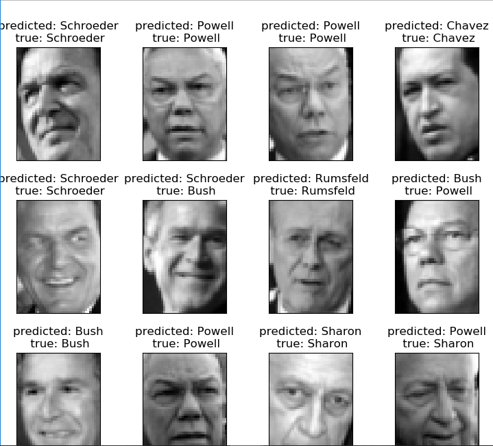
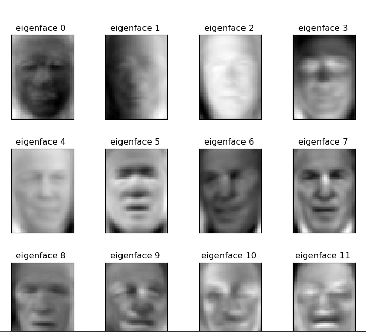
下面这个是用主成分分析提取特征后的图像

两个矩阵的解释

precision recall f1-score support

avg / total 0.85 0.85 0.85 322

这个

- TP，True Positive 本来是对的也预测对了
- FP，False Positive 本来是对的但预测错了
- TN，True Negative 本来是错的也预测对了
- FN，False Negative 本来是错了但是也预测错了

precision = TP / (TP + FP)

recall = TP / (TP + FN)

accuracy = (TP + TN) / (TP + FP + TN + FN)

F1 Score = P*R/2(P+R)，其中P和R分别为 precision 和 recall

[[ 12 3 0 0 0 0 0]
[ 1 51 0 5 0 0 2]
[ 2 1 30 2 0 1 1]
[ 1 5 5 120 2 0 1]
[ 0 1 0 2 23 0 2]
[ 0 1 0 1 0 12 0]
[ 0 1 0 4 5 0 25]]

就是七个类，7*7的矩阵，一个类被预测为的类加一，明显对角线是预测为本身的数量。最多

其中一些函数的具体解释

lfw_people=fetch_lfw_people(min_faces_per_person=70,resize=0.4)

'''
看他的官方文档
def fetch_lfw_people(data_home=None, funneled=True, resize=0.5,
min_faces_per_person=0, color=False,
slice_=(slice(70, 195), slice(78, 172)),
download_if_missing=True):
"""Loader for the Labeled Faces in the Wild (LFW) people dataset

This dataset is a collection of JPEG pictures of famous people
collected on the internet, all details are available on the
official website:

http://vis-www.cs.umass.edu/lfw/

Each picture is centered on a single face. Each pixel of each channel
(color in RGB) is encoded by a float in range 0.0 - 1.0.

The task is called Face Recognition (or Identification): given the
picture of a face, find the name of the person given a training set
(gallery).
The original images are 250 x 250 pixels, but the default slice and resize
arguments reduce them to 62 x 74.

Parameters
----------
data_home : optional, default: None
Specify another download and cache folder for the datasets. By default
all scikit learn data is stored in '~/scikit_learn_data' subfolders.

funneled : boolean, optional, default: True
Download and use the funneled variant of the dataset.
resize : float, optional, default 0.5
Ratio used to resize the each face picture.

min_faces_per_person : int, optional, default None
The extracted dataset will only retain pictures of people that have at
least `min_faces_per_person` different pictures.

color : boolean, optional, default False
Keep the 3 RGB channels instead of averaging them to a single
gray level channel. If color is True the shape of the data has
one more dimension than the shape with color = False.

slice_ : optional
Provide a custom 2D slice (height, width) to extract the
'interesting' part of the jpeg files and avoid use statistical
correlation from the background

download_if_missing : optional, True by default
If False, raise a IOError if the data is not locally available
instead of trying to download the data from the source site.

Returns
-------
dataset : dict-like object with the following attributes:

dataset.data : numpy array of shape (13233, 2914)
Each row corresponds to a ravelled face image of original size 62 x 47
pixels. Changing the ``slice_`` or resize parameters will change the
shape of the output.

dataset.images : numpy array of shape (13233, 62, 47)
Each row is a face image corresponding to one of the 5749 people in
the dataset. Changing the ``slice_`` or resize parameters will change
the shape of the output.

dataset.target : numpy array of shape (13233,)
Labels associated to each face image. Those labels range from 0-5748
and correspond to the person IDs.

dataset.DESCR : string
Description of the Labeled Faces in the Wild (LFW) dataset

意思就是min_faces_per_person=定义了每个人取多少个不同图片,resize=重新定义了图片的大小
'''


pca=PCA(svd_solver='randomized',n_components=n_components,whiten=True).fit(X_train)

'''
n_components:PCA算法中所要保留的主成分个数n，也即保留下来的特征个数n
类型：int 或者 string，缺省时默认为None，所有成分被保留。
          赋值为int，比如n_components=1，将把原始数据降到一个维度。
          赋值为string，比如n_components='mle'，将自动选取特征个数n，使得满足所要求的方差百分比。
          
copy:表示是否在运行算法时，将原始训练数据复制一份。若为True，则运行PCA算法后，原始训练数据的值不会有任何改变，因为是在原始数据的副本上进行运算；若为False，则运行PCA算法后，原始训练数据的值会改，因为是在原始数据上进行降维计算。
类型：bool，True或者False，缺省时默认为True。

whiten:白化，使得每个特征具有相同的方差。由于图像中相邻像素之间具有很强的相关性，所以用于训练时输入是冗余的。白化的目的就是降低输入的冗余性；更正式的说，我们希望通过白化过程使得学习算法的输入具有如下性质：(i)特征之间相关性较低；(ii)所有特征具有相同的方差。

类型：bool，缺省时默认为False

PCA对象的属性
components_ ：返回具有最大方差的成分。
explained_variance_ratio_：返回 所保留的n个成分各自的方差百分比。
n_components_：返回所保留的成分个数n。
mean_：
noise_variance_：

'''

很容易理解。用的时候再具体看。

同时我照着教程上的代码写的时候也遇到了一些错误

1、 DeprecationWarning: This module was deprecated in version 0.18 in favor of the model_selection module into which all the refactored classes and functions are moved. This module will be removed in 0.20.
DeprecationWarning)
该模块在0.18版本中被弃用，支持所有重构的类和函数都被移动到的model_selection模块

解决办法。

将

from sklearn.model_selection import GridSearchCV

from sklearn.model_selection import train_test_split

改为：
from sklearn.grid_search import GridSearchCV

from sklearn.cross_validation import train_test_split

2、ValueError: class_weight must be dict, 'balanced', or None, got: 'auto'

在第五十行

clf = GridSearchCV(SVC(kernel='rbf'),param_grid)中原本是clf = GridSearchCV(SVC(kernel='rbf',class_weight ='auto'),param_grid).但是

class_weight ='auto'在此版本中不存在，删除即可。或者用 'balanced' or None

3、DeprecationWarning: Class RandomizedPCA is deprecated; RandomizedPCA was deprecated in 0.18 and will be removed in 0.20. Use PCA(svd_solver='randomized') instead. The new implementation DOES NOT store whiten ``components_``. Apply transform to get them.
warnings.warn(msg, category=DeprecationWarning)

还是版本问题
将from sklearn.decomposition import RandomizedPCA修改为from sklearn.decomposition import PCA

然后将出错的那个程序句子改为：pca = PCA(svd_solver='randomized', n_components = n_components, whiten = True).fit(X_train)即可

4、ValueError: Found input variables with inconsistent numbers of samples: [322, 966]

两个矩阵行或者宽的不一样而已，我打错了。

今天也只是入个门。学的还不是太深。今后有机会会继续深入学习的。

在此推荐个大佬写的

支持向量机原理(一) 线性支持向量机

支持向量机原理(二) 线性支持向量机的软间隔最大化模型

支持向量机原理(三)线性不可分支持向量机与核函数

支持向量机原理(四)SMO算法原理

支持向量机原理(五)线性支持回归

有空一定要研究一下。

另外，我看到网上也有很多写的跟我一样的博客。学的教程都一样。有的只是简单复制粘贴，有的也写的很详细。我想说的是，既然学了就学的尽量详细点，也就是代码自己一句一句的打，每个函数都弄清楚。算法原理也要及时记下来。不要只看看教程看看别人实现一遍。

$ξ_{i} \geq 0$