# 通过网格搜索、学习曲线对泰坦尼克号数据集调参

在这里下载数据集
导入模块

import numpy as np
import pandas as pd
import seaborn as sns
from scipy import stats,integrate
import matplotlib.pyplot as plt
%matplotlib inline
titanic=pd.read_csv("train.csv")

数据预处理

# 正则表达式模块
import re

# 由于年龄中有空值，需要先用平均值对年龄的缺失值进行填充，因为矩阵运算只能是数值型，不能是字符串
titanic['Age'] = titanic['Age'].fillna(titanic['Age'].mean())
# 同理，由于Embarked（登船地点）里面也有空值，所以也需要用出现最多的类型对它进行一个填充
titanic['Embarked'] = titanic['Embarked'].fillna('S')

# 对于性别中的male与female，用0和1来表示。首先看性别是否只有两个值
# 对于登船地点的三个值S C Q，也用0 1 2分别表示
# print(titanic['Sex'].unique())
# print(titanic['Embarked'].unique())
titanic.loc[titanic['Sex'] == 'male', 'Sex'] = 0
titanic.loc[titanic['Sex'] == 'female', 'Sex'] = 1

titanic.loc[titanic['Embarked'] == 'S', 'Embarked'] = 0
titanic.loc[titanic['Embarked'] == 'C', 'Embarked'] = 1
titanic.loc[titanic['Embarked'] == 'Q', 'Embarked'] = 2

# 加上其余的属性特性
titanic["FamilySize"] = titanic["SibSp"] + titanic["Parch"]

# 姓名的长度
titanic["NameLenght"] = titanic["Name"].apply(lambda x: len(x))


# 定义提取姓名中Mr以及Mrs等属性
def get_title(name):
    title_search = re.search(' ([A-Za-z]+)\.', name)
    if title_search:
        return title_search.group(1)
    return ""


titles = titanic["Name"].apply(get_title)
# 对于姓名中的一些称呼赋予不同的数值
title_mapping = {'Mr': 1, 'Miss': 2, 'Mrs': 3, 'Master': 4, 'Dr': 5, 'Rev': 6, 'Major': 7, 'Mlle': 8, 'Col': 9,
                 'Capt': 10, 'Ms': 11, 'Don': 12, 'Jonkheer': 13, 'Countess': '14', 'Lady': 15, 'Sir': 16, 'Mme': 17}
for k,v in title_mapping.items():
    titles[titles == k] = v
titanic['Titles'] = titles

通过图表显示数据

# 导入图表函数
import matplotlib.pyplot as plt
import pandas
from pylab import *
# 图表汉字正常显示
mpl.rcParams['font.sans-serif'] = ['SimHei']
# 图表负值正常显示
matplotlib.rcParams['axes.unicode_minus'] = False

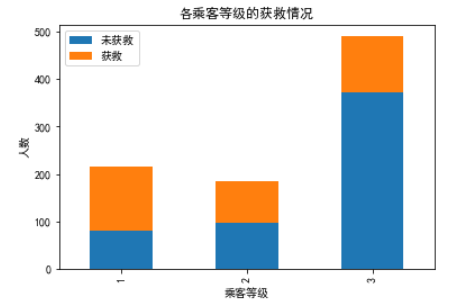
# 查看各等级乘客等级的获救情况
fig = plt.figure()
# 设置图表颜色的alpha参数
fig.set(alpha=0.2)

Suvived_0 = titanic.Pclass[titanic.Survived == 0].value_counts()
Suvived_1 = titanic.Pclass[titanic.Survived == 1].value_counts()
df = pandas.DataFrame({u"获救": Suvived_1, u"未获救": Suvived_0})
df.plot(kind='bar', stacked=True)
plt.title(u'各乘客等级的获救情况')
plt.xlabel(u'乘客等级')
plt.ylabel(u'人数')
plt.show()

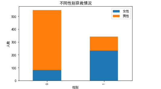
# 按性别分组
fig = plt.figure()
fig.set(alpha=0.2)

Survived_m = titanic.Survived[titanic.Sex == 0].value_counts()
Survived_f = titanic.Survived[titanic.Sex == 1].value_counts()
df = pandas.DataFrame({u'男性': Survived_m, u'女性': Survived_f})
df.plot(kind='bar', stacked=True)
plt.title(u'不同性别获救情况')
plt.xlabel(u'性别')
plt.ylabel(u'人数')
plt.show()

随机森林预测

# 导入随机森林模型
from sklearn.ensemble import RandomForestClassifier
from sklearn.model_selection import cross_val_score
alg = RandomForestClassifier(random_state=1, n_estimators=100, min_samples_split=4, min_samples_leaf=2)
presictors = ["Pclass", "Sex", "Age", "SibSp", "Parch", "Fare", "Embarked", "Titles", "FamilySize", "NameLenght"]
scores = cross_val_score(alg, titanic[presictors], titanic["Survived"], cv=10).mean()
print(scores.mean())

0.8316311996368176

进行调参，先调n_estimators

scorel = []
for i in range(0,200,10):
    alg = RandomForestClassifier(n_estimators=i+1,n_jobs=-1,random_state=1)
    score = cross_val_score(alg, titanic[presictors], titanic["Survived"], cv=10).mean()
    scorel.append(score)
print(max(scorel),(scorel.index(max(scorel))*10)+1)
plt.figure(figsize=[20,5])
plt.plot(range(1,201,10),scorel)
plt.show()

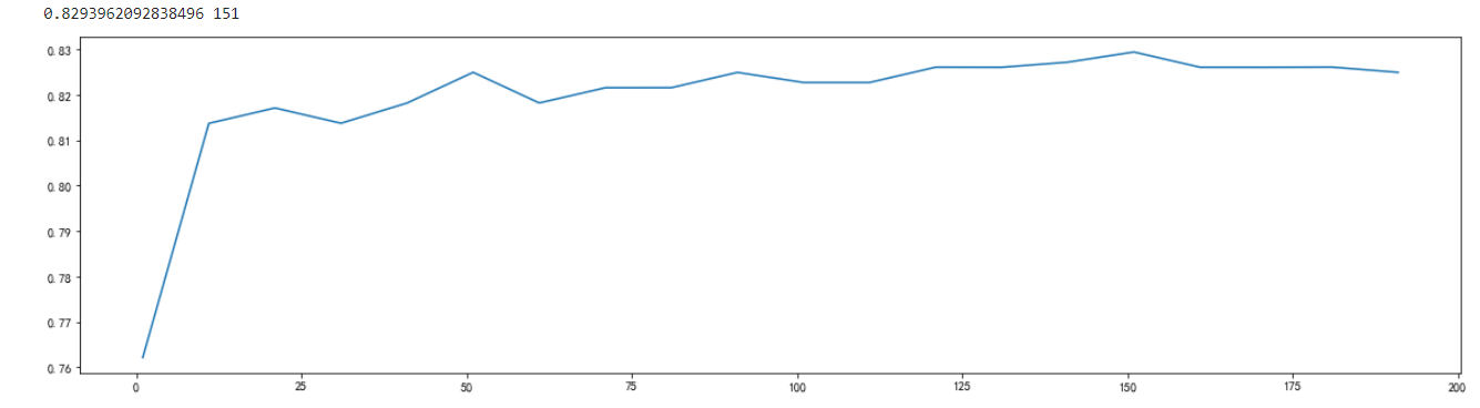
进行细化,得到当n_estimators为145时，准确率最高

scorel = []
for i in range(145,155):
    alg = RandomForestClassifier(n_estimators=i+1,n_jobs=-1,random_state=1)
    score = cross_val_score(alg, titanic[presictors], titanic["Survived"], cv=10).mean()
    scorel.append(score)
print(max(scorel),([*range(145,155)][scorel.index(max(scorel))]))
plt.figure(figsize=[20,5])
plt.plot(range(145,155),scorel)
plt.show()

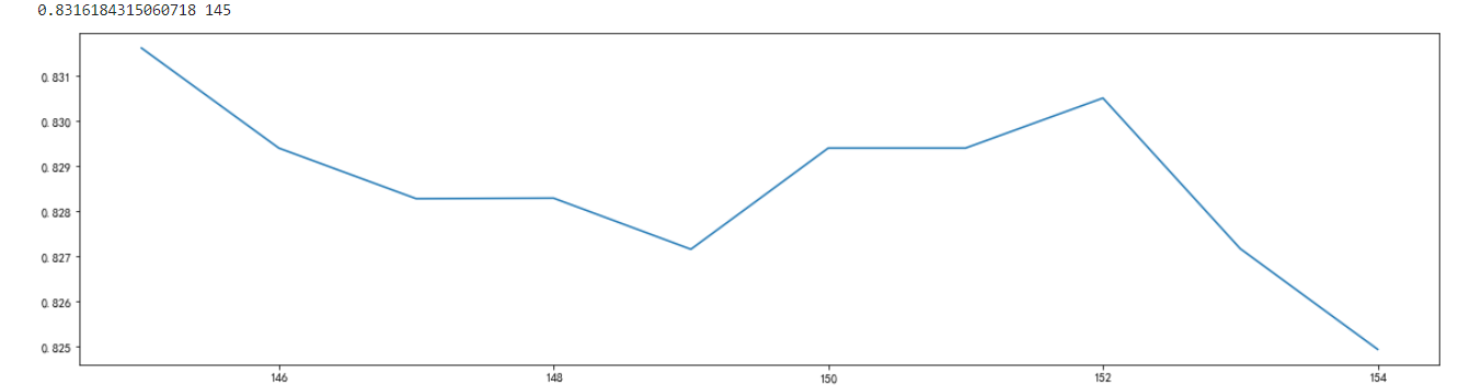
确定n_estimators，开始进一步调整max_depth

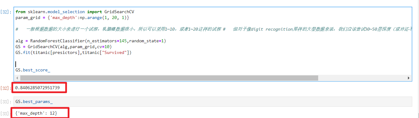
from sklearn.model_selection import GridSearchCV
param_grid = {'max_depth':np.arange(1, 20, 1)}
 
#   一般根据数据的大小来进行一个试探，乳腺癌数据很小，所以可以采用1~10，或者1~20这样的试探 #   但对于像digit recognition那样的大型数据来说，我们应该尝试30~50层深度（或许还不足够 #   更应该画出学习曲线，来观察深度对模型的影响
 
alg = RandomForestClassifier(n_estimators=145,random_state=1) 
GS = GridSearchCV(alg,param_grid,cv=10) 
GS.fit(titanic[presictors],titanic["Survived"])
GS.best_score_

得到当深度为12时，准确率达到84%

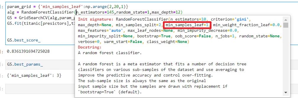
继续调整min_samples_leaf，当它为3时学习率为83.6%，不增反降，以随机森林为代表的装袋法的训练过程旨在降低方差，即降低模型复杂度，所以随机森林参数的默认设定都是假设模型本身在泛化误差最低点的右边，min_samples_leaf最佳值为1

param_grid = {'min_samples_leaf':np.arange(2,20,1)}
alg = RandomForestClassifier(n_estimators=145,random_state=1,max_depth=12) 
GS = GridSearchCV(alg,param_grid,cv=10) 
GS.fit(titanic[presictors],titanic["Survived"])
GS.best_score_

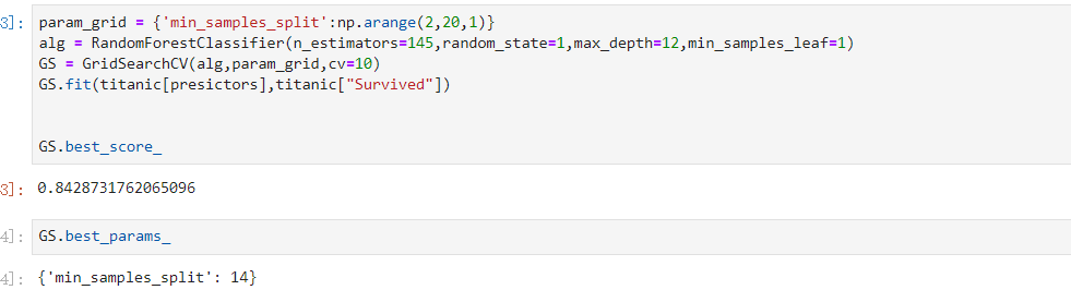
继续调min_samples_split,它为14

param_grid = {'min_samples_split':np.arange(2,20,1)}
alg = RandomForestClassifier(n_estimators=145,random_state=1,max_depth=12,min_samples_leaf=1) 
GS = GridSearchCV(alg,param_grid,cv=10) 
GS.fit(titanic[presictors],titanic["Survived"])
GS.best_score_

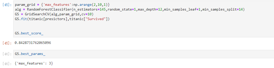
继续调max_features，它为3时，准确率最高和上面的准确率一致

param_grid = {'max_features':np.arange(2,10,1)}
alg = RandomForestClassifier(n_estimators=145,random_state=1,max_depth=12,min_samples_leaf=1,min_samples_split=14) 
GS = GridSearchCV(alg,param_grid,cv=10) 
GS.fit(titanic[presictors],titanic["Survived"])
GS.best_score_

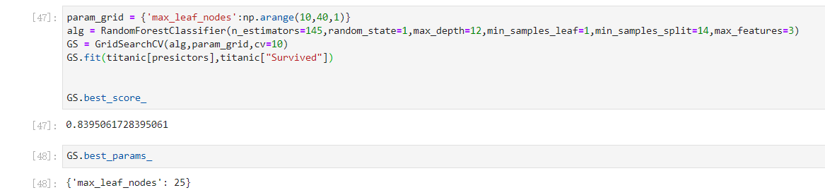
再调max_leaf_nodes，发现不增反降，说明学习率在上面的情况已经到达了最好

param_grid = {'max_leaf_nodes':np.arange(10,40,1)}
alg = RandomForestClassifier(n_estimators=145,random_state=1,max_depth=12,min_samples_leaf=1,min_samples_split=14,max_features=3) 
GS = GridSearchCV(alg,param_grid,cv=10) 
GS.fit(titanic[presictors],titanic["Survived"])
GS.best_score_

最后调好的参数如下，比开始提升了0.011235955056179692:

alg = RandomForestClassifier(n_estimators=145,random_state=1,max_depth=12,min_samples_leaf=1,min_samples_split=14,max_features=3) 
score = cross_val_score(alg,titanic[presictors],titanic["Survived"],cv=10).mean() 
score-scores

参考链接：
https://www.cnblogs.com/SUNYZBlog/p/9695399.html