Tensorflow读书笔记

第六章

(1)卷积中的局部连接：层间神经只有局部范围内的连接，在这个范围内采用全连接的方式，超过这个范围的神经元则没有连接；连接与连接之间独立参数，相比于去全连接减少了感受域外的连接，有效减少参数规模。

全连接：层间神经元完全连接，每个输出神经元可以获取到所有神经元的信息，有利于信息汇总，常置于网络末尾；连接与连接之间独立参数，大量的连接大大增加模型的参数规模。

（3）池化的作用：对输入的特征图进行压缩，一方面使特征图变小，简化网络计算复杂度；一方面进行特征压缩，提取主要特征。

激活函数的作用：如果不用激励函数，每一层输出都是上层输入的线性函数，无论神经网络有多少层，输出都是输入的线性组合。

（4）归一化有助于快速收敛；对局部神经元的活动创建竞争机制，使得其中响应比较大的值变得相对更大，并抑制其他反馈较小的神经元，增强了模型的泛化能力。

（5）寻找损失函数的最低点，就像我们在山谷里行走，希望找到山谷里最低的地方。那么如何寻找损失函数的最低点呢？在这里，我们使用了微积分里导数，通过求出函数导数的值，从而找到函数下降的方向或者是最低点（极值点）。损失函数里一般有两种参数，一种是控输入信号量的权重，另一种是调整函数与真实值距离的偏差。我们所要做的工作，就是通过梯度下降方法，不断地调整权重 和偏差b，使得损失函数的值变得越来越小。

 

 

import tensorflow as tf
from tensorflow import keras
import numpy as np
import matplotlib.pyplot as plt
fashion_mnist=keras.datasets.fashion_mnist
(train_images,train_labels),(test_images,test_labels)=fashion_mnist.load_data()
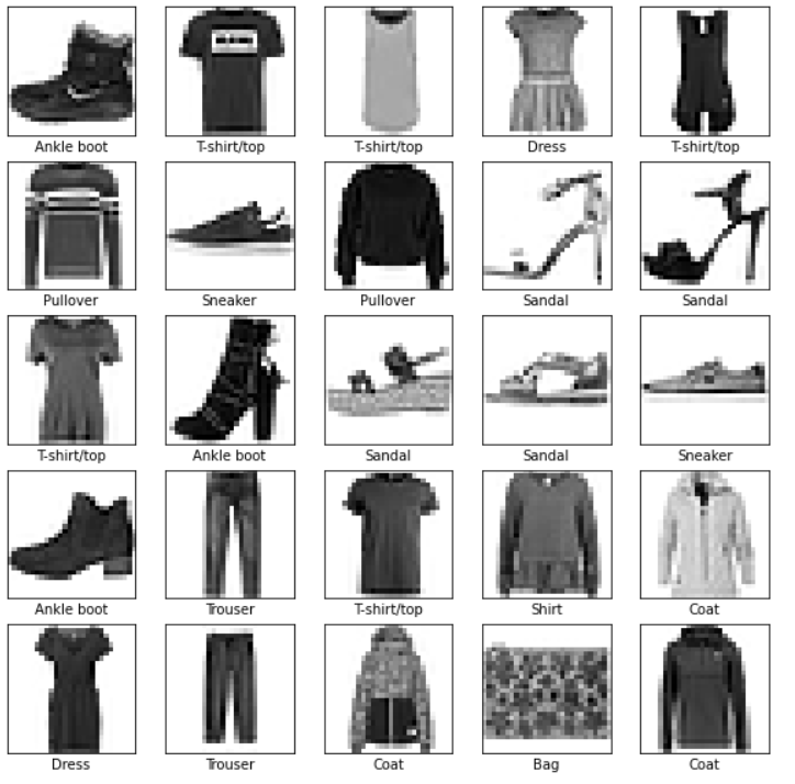
class_names=['T-shirt/top','Trouser','Pullover','Dress','Coat','Sandal','Shirt','Sneaker','Bag','Ankle boot']
train_labels
train_images.shape
len(train_labels)
test_images.shape
len(test_labels)
plt.figure()
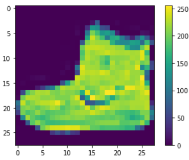
plt.imshow(train_images[0])
plt.colorbar()
plt.grid(False)
plt.show()
train_images=train_images/255.0
test_images=test_images/255.0
plt.figure(figsize=(10,10))
for i in range(25):
plt.subplot(5,5,i+1)
plt.xticks([])
plt.yticks([])
plt.grid(False)
plt.imshow(train_images[i],cmap=plt.cm.binary)
plt.xlabel(class_names[train_labels[i]])
plt.show()
model=keras.Sequential([
keras.layers.Flatten(input_shape=(28,28)),
keras.layers.Dense(128,activation='relu'),
keras.layers.Dense(10)])
model.compile(optimizer='adam',
loss=tf.keras.losses.SparseCategoricalCrossentropy(from_logits=True),
metrics=['accuracy'])
model.fit(train_images,train_labels,epochs=10)
test_loss,test_acc=model.evaluate(test_images,test_labels,verbose=2)
print('\nTest accuracy:',test_acc)
probability_model=tf.keras.Sequential([model,
tf.keras.layers.Softmax()])
predictions=probability_model.predict(test_images)
predictions[0]
np.argmax(predictions[0])
test_labels[0]
def plot_image(i,predictions_array,true_label,img):
predictions_array, true_label, img=predictions_array, true_label[i], img[i]
plt.grid(False)
plt.xticks([])
plt.yticks([])
plt.imshow(img, cmap=plt.cm.binary)
predicted_label = np.argmax(predictions_array)
if predicted_label == true_label:
color = 'blue'
else:
color = 'red'

plt.xlabel("{} {:2.0f}% ({})".format(class_names[predicted_label],
100*np.max(predictions_array),
class_names[true_label]),
color=color)

def plot_value_array(i, predictions_array, true_label):
predictions_array, true_label = predictions_array, true_label[i]
plt.grid(False)
plt.xticks(range(10))
plt.yticks([])
thisplot = plt.bar(range(10), predictions_array, color="#777777")
plt.ylim([0, 1])
predicted_label = np.argmax(predictions_array)

thisplot[predicted_label].set_color('red')
thisplot[true_label].set_color('blue')
i = 0
plt.figure(figsize=(6,3))
plt.subplot(1,2,1)
plot_image(i, predictions[i], test_labels, test_images)
plt.subplot(1,2,2)
plot_value_array(i,predictions[i],test_labels)
plt.show()
# Plot the first X test images, their predicted labels, and the true labels.
# Color correct predictions in blue and incorrect predictions in red.
num_rows = 5
num_cols = 3
num_images = num_rows*num_cols
plt.figure(figsize=(2*2*num_cols, 2*num_rows))
for i in range(num_images):
plt.subplot(num_rows,2*num_cols,2*i+1)
plot_image(i, predictions[i], test_labels, test_images)
plt.subplot(num_rows, 2*num_cols, 2*i+2)
plot_value_array(i, predictions[i], test_labels)
plt.tight_layout()
plt.show()
#测试部分
img=test_images[1]
print(img.shape)
img=(np.expand_dims(img,0))
print(img.shape)
predictions_single=probability_model.predict(img)
print(predictions_single)
plot_value_array(1,predictions_single[0],test_labels)
_ =plt.xticks(range(10),class_names,rotation=45)
np.argmax(predictions_single[0])

 

# 导入所需模块
import tensorflow as tf
from sklearn import datasets
from matplotlib import pyplot as plt
%matplotlib inline
import numpy as np

# 导入数据，分别为输入特征和标签
x_data = datasets.load_iris().data
y_data = datasets.load_iris().target

# 随机打乱数据（因为原始数据是顺序的，顺序不打乱会影响准确率）
# seed: 随机数种子，是一个整数，当设置之后，每次生成的随机数都一样（为方便教学，以保每位同学结果一致）
np.random.seed(116)  # 使用相同的seed，保证输入特征和标签一一对应
np.random.shuffle(x_data)
np.random.seed(116)
np.random.shuffle(y_data)
tf.random.set_seed(116)

# 将打乱后的数据集分割为训练集和测试集，训练集为前120行，测试集为后30行
x_train = x_data[:-30]
y_train = y_data[:-30]
x_test = x_data[-30:]
y_test = y_data[-30:]

# 转换x的数据类型，否则后面矩阵相乘时会因数据类型不一致报错
x_train = tf.cast(x_train, tf.float32)
x_test = tf.cast(x_test, tf.float32)

# from_tensor_slices函数使输入特征和标签值一一对应。（把数据集分批次，每个批次batch组数据）
train_db = tf.data.Dataset.from_tensor_slices((x_train, y_train)).batch(32)
test_db = tf.data.Dataset.from_tensor_slices((x_test, y_test)).batch(32)

# 生成神经网络的参数，4个输入特征故，输入层为4个输入节点；因为3分类，故输出层为3个神经元
# 用tf.Variable()标记参数可训练
# 使用seed使每次生成的随机数相同（方便教学，使大家结果都一致，在现实使用时不写seed）
w1 = tf.Variable(tf.random.truncated_normal([4, 3], stddev=0.1, seed=1))
b1 = tf.Variable(tf.random.truncated_normal([3], stddev=0.1, seed=1))

#定义超参数
lr = 0.1  # 学习率为0.1
train_loss_results = []  # 将每轮的loss记录在此列表中，为后续画loss曲线提供数据
test_acc = []  # 将每轮的acc记录在此列表中，为后续画acc曲线提供数据
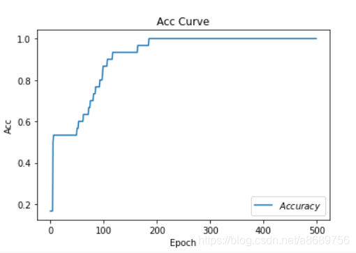
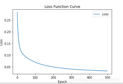
epoch = 500  # 循环500轮
loss_all = 0  # 每轮分4个step，loss_all记录四个step生成的4个loss的和

# 训练部分
for epoch in range(epoch):  #数据集级别的循环，每个epoch循环一次数据集
    for step, (x_train, y_train) in enumerate(train_db):  #batch级别的循环 ，每个step循环一个batch
        with tf.GradientTape() as tape:  # with结构记录梯度信息
            y = tf.matmul(x_train, w1) + b1  # 神经网络乘加运算
            y = tf.nn.softmax(y)  # 使输出y符合概率分布（此操作后与独热码同量级，可相减求loss）
            y_ = tf.one_hot(y_train, depth=3)  # 将标签值转换为独热码格式，方便计算loss和accuracy
            loss = tf.reduce_mean(tf.square(y_ - y))  # 采用均方误差损失函数mse = mean(sum(y-out)^2)
            loss_all += loss.numpy()  # 将每个step计算出的loss累加，为后续求loss平均值提供数据，这样计算的loss更准确
        # 计算loss对各个参数的梯度
        grads = tape.gradient(loss, [w1, b1])

        # 实现梯度更新 w1 = w1 - lr * w1_grad    b = b - lr * b_grad
        w1.assign_sub(lr * grads[0])  # 参数w1自更新
        b1.assign_sub(lr * grads[1])  # 参数b自更新

    # 每个epoch，打印loss信息
    print("Epoch {}, loss: {}".format(epoch, loss_all/4))
    train_loss_results.append(loss_all / 4)  # 将4个step的loss求平均记录在此变量中
    loss_all = 0  # loss_all归零，为记录下一个epoch的loss做准备

    # 测试部分
    # total_correct为预测对的样本个数, total_number为测试的总样本数，将这两个变量都初始化为0
    total_correct, total_number = 0, 0
    for x_test, y_test in test_db:
        # 使用更新后的参数进行预测
        y = tf.matmul(x_test, w1) + b1#计算前向传播预测结果
        y = tf.nn.softmax(y)#变为概率分布
        pred = tf.argmax(y, axis=1)  # 返回y中最大值的索引，即预测的分类
        # 将pred转换为y_test的数据类型
        pred = tf.cast(pred, dtype=y_test.dtype)
        # 若分类正确，则correct=1，否则为0，将bool型的结果转换为int型
        correct = tf.cast(tf.equal(pred, y_test), dtype=tf.int32)
        # 将每个batch的correct数加起来
        correct = tf.reduce_sum(correct)
        # 将所有batch中的correct数加起来
        total_correct += int(correct)
        # total_number为测试的总样本数，也就是x_test的行数，shape[0]返回变量的行数
        total_number += x_test.shape[0]
    # 总的准确率等于total_correct/total_number
    acc = total_correct / total_number
    test_acc.append(acc)
    print("Test_acc:", acc)
    print("--------------------------")

# 绘制 loss 曲线
plt.title('Loss Function Curve')  # 图片标题
plt.xlabel('Epoch')  # x轴变量名称
plt.ylabel('Loss')  # y轴变量名称
plt.plot(train_loss_results, label="$Loss$")  # 逐点画出trian_loss_results值并连线，连线图标是Loss
plt.legend()  # 画出曲线图标
plt.show()  # 画出图像

# 绘制 Accuracy 曲线
plt.title('Acc Curve')  # 图片标题
plt.xlabel('Epoch')  # x轴变量名称
plt.ylabel('Acc')  # y轴变量名称
plt.plot(test_acc, label="$Accuracy$")  # 逐点画出test_acc值并连线，连线图标是Accuracy
plt.legend()
plt.show()

 

 

读书笔记：

梯度下降、随机梯度下降和批梯度下降
一、梯度下降
(1) 如果数据集比较小，完全可以采用全数据集(Full Batch Learning)的形式，采用全数据有两个好处：
a. 由全数据集确定的方向能够更好地代表样本总体，从而更准确地朝向极值所在的方向。
b. 由于不同权重的梯度值差别巨大，因此选取一个全局的学习率很困难。 Full Batch Learning 可以使用 Rprop 只基于梯度符号并且针对性单独更新各权值。
(2) 但是梯度下降也存在一下这些缺点：
a. 梯度下降算法并不能保证被优化函数达到全局最优解，只有当损失函数为凸函数时,梯度下降算法才能保证达到全局最优解，因此不能保证一定达到全局最优，受限于损失函数是否为凸函数。
b. 梯度下降算法的另外一个问题是计算时间太长，因为要在全部训练数据上最小化损失，在海量训练数据下，这样是十分耗时。
二. 随机梯度下降算法:
为了加速训练的过程，可以使用随机梯度下降算法(stochastic gradient descent-SGD)。随机梯度下降算法也是称为"在线学习"。
(1) 这个算法优化的不是在全部训练数据上的损失函数，而是在每轮迭代中，随机优化某一条训练数据上的损失函数，这样每一轮参数的更新速度大大加快。
(2) 但是带来了如下问题：
在某一条数据上损失函数更小并不代表在全部数据上的损失函数更小，于是使用随机梯度下降优化得到的神经网络甚至可能无法达到全局最优。
三. 批梯度下降算法：
为了综合梯度下降算法和随机梯度下降算法的优缺点，在实际应用中一般采用这两个算法的这种----->每次计算一小部分训练数据的损失函数。批梯度下降算法（Mini-batches Learning）在深度学习很多算法的反向传播算法中非常常用。这一小部分训练数据也称为一个batch，因此也引入了batch_size的概念，batch_size顾名思义就是来度量每一个batch中实例的个数。
(1) 引入batch有很好的优势：
a. 通过矩阵运算，每次在一个batch上优化神经网络参数并不会比单个数据慢太多。
b. 每次使用一个batch可以大大减小收敛所需要的迭代次数，同时可以使收敛到的结果更加接近梯度下降的效果。
--->但是批梯度下降算法带来一个问题，那就是如何选取最优的batch_size?
(2) 可不可以选择一个适中的 Batch_Size 值呢？
当然可以，这就是批梯度下降法(Mini-batches Learning)。因为如果数据集足够充分，那么用一半(甚至少得多)的数据训练算出来的梯度与用全部数据训练出来的梯度是几乎一样的。
(3) 在合理范围内，增大 Batch_Size 有何好处？
a. 内存利用率提高了，大矩阵乘法的并行化效率提高。
b. 跑完一次 epoch（全数据集）所需的迭代次数减少，对于相同数据量的处理速度进一步加快。
c. 在一定范围内，一般来说 Batch_Size 越大，其确定的下降方向越准，引起训练震荡越小。
(4) 盲目增大 Batch_Size 有何坏处？
a. 内存利用率提高了，但是内存容量可能撑不住了。
b. 跑完一次 epoch（全数据集）所需的迭代次数减少，要想达到相同的精度，其所花费的时间大大增加了，从而对参数的修正也就显得更加缓慢。
c. Batch_Size 增大到一定程度，其确定的下降方向已经基本不再变化。

 

TensorFlow常用的优化函数
tf.train.Optimizer
tf.train.GradientDescentOptimizer
tf.train.AdadeltaOptimizer
tf.train.AdagtadOptimizer
tf.train.AdagradDAOptimizer
tf.train.MomentumOptimizer
tf.train.AdamOptimizer
tf.train.FtrlOptimizer
tf.train.ProximalGradientDescentOptimizer
tf.train.ProximalAdagradOptimizer
tf.train.RMSProOptimizer