智能电网的电能预估及价值分析

智能电网的电能预估及价值分析

一、实验目的与要求
1、掌握使用pandas库处理数据的基本方法。
2、掌握对时间序列类数据预处理的基本方法。
3、掌握使用matplotlib结合pandas库对数据分析可视化处理的基本方法。
二、实验内容
1、利用python中pandas等库读取数据，并完成数据的预处理。
2、利用matplotlib等库完成对数据的可视化。
3、使用Sklearn库的相关系数建立决策树模型，对模型进行训练，使用测试集测试后对模型的效果进行评价。
三、实验步骤

1.数据预处理。读取所提供的数据文件，检查文件中时间序列是否完整，有无缺失值，重复值。

（1）导入所需要使用的包

import os
import numpy as np
import pandas as pd 
import matplotlib.pyplot as plt
import matplotlib.dates as mdate
from datetime import datetime, timedelta
from matplotlib.dates import DateFormatter, WeekdayLocator, DayLocator, MONDAY,YEARLY
import dateutil.relativedelta
import time
from matplotlib.pyplot import MultipleLocator
from pandas.core.common import SettingWithCopyWarning
from sklearn import tree#决策树模型
from sklearn.model_selection import train_test_split#划分测试集合与训练集合
from sklearn.model_selection import GridSearchCV#用于找到最优模型
from scipy.stats import pearsonr
from sklearn.tree import DecisionTreeRegressor
#设置字体
plt.rcParams['font.sans-serif']=['SimHei']

（2）读取文件

file_path='/data/bigfiles/data3.csv'
data=pd.read_csv(file_path)

（3）查看数据的基本统计信息

data.info()

<class 'pandas.core.frame.DataFrame'>
RangeIndex: 87648 entries, 0 to 87647
Data columns (total 8 columns):
日期      87648 non-null object
小时      87648 non-null float64
干球温度    87648 non-null float64
露点温度    87648 non-null float64
湿球温度    87648 non-null float64
湿度      87648 non-null float64
电价      87648 non-null float64
电力负荷    87648 non-null float64
dtypes: float64(7), object(1)
memory usage: 5.3+ MB

（4）检查数据是否完整

# 查看数据长度
std_rng=pd.date_range(start='2006/1/1',end='2011/1/1',freq='D')
len(std_rng)

1827

（5）求日平均数据并添加日类型

data['湿度']=data['湿度'].map(lambda x :float(x))

#湿度转换成 浮点类型
data['日最高湿度']=data["湿度"]
data['日最低湿度']=data["湿度"]
data['日均电力负荷']=data['电力负荷']
data['日最高电力负荷']=data['电力负荷']
data['日最低电力负荷']=data['电力负荷']

# 将日期设为行索引
data=data.set_index(['日期'])
data

	小时	干球温度	露点温度	湿球温度	湿度	电价	电力负荷	日最高湿度	日最低湿度	日均电力负荷	日最高电力负荷	日最低电力负荷
日期
2006/1/1	0.5	23.90	21.65	22.40	87.5	19.67	8013.27833	87.5	87.5	8013.27833	8013.27833	8013.27833
2006/1/1	1.0	23.90	21.70	22.40	88.0	18.56	7726.89167	88.0	88.0	7726.89167	7726.89167	7726.89167
2006/1/1	1.5	23.80	21.65	22.35	88.0	19.09	7372.85833	88.0	88.0	7372.85833	7372.85833	7372.85833
2006/1/1	2.0	23.70	21.60	22.30	88.0	17.40	7071.83333	88.0	88.0	7071.83333	7071.83333	7071.83333
2006/1/1	2.5	23.70	21.60	22.30	88.0	17.00	6865.44000	88.0	88.0	6865.44000	6865.44000	6865.44000
...	...	...	...	...	...	...	...	...	...	...	...	...
2010/12/31	22.0	22.60	19.10	20.40	81.0	23.86	8449.54000	81.0	81.0	8449.54000	8449.54000	8449.54000
2010/12/31	22.5	22.45	19.05	20.30	81.5	26.49	8508.16000	81.5	81.5	8508.16000	8508.16000	8508.16000
2010/12/31	23.0	22.30	19.00	20.20	82.0	25.18	8413.14000	82.0	82.0	8413.14000	8413.14000	8413.14000
2010/12/31	23.5	22.05	19.05	20.15	83.5	26.19	8173.79000	83.5	83.5	8173.79000	8173.79000	8173.79000
2011/1/1	0.0	21.80	19.10	20.10	85.0	24.62	8063.36000	85.0	85.0	8063.36000	8063.36000	8063.36000

87648 rows × 12 columns

# 将日期类型转换成datatime
data.index=data.index.map(lambda x :datetime.strptime(x,'%Y/%m/%d'))
data['日']=data.index

# 定义中文包
week_cn = [1,2,3,4,5,6,7]
data['日']=data['日'].map(lambda x: week_cn[pd.to_datetime(x).weekday()])

datas =data.groupby('日期').agg({"干球温度":"mean","露点温度":"mean","湿球温度":"mean","湿度":"mean","日最高湿度":"max","日最低湿度":"min","电价":"mean","日最高电力负荷":"max","日最低电力负荷":"min","日均电力负荷":"mean","日":"mean"})
# 对缺失的值进行填补
datas.head(30)

	干球温度	露点温度	湿球温度	湿度	日最高湿度	日最低湿度	电价	日最高电力负荷	日最低电力负荷	日均电力负荷	日
日期
2006-01-01	32.790426	16.987234	22.910638	50.244681	90.0	15.0	43.721702	11112.76333	6388.27833	9188.743865	7
2006-01-02	20.855208	17.447917	18.757292	81.072917	92.0	73.0	16.273542	8456.72833	6364.80333	7686.274860	1
2006-01-03	23.122917	16.632292	19.172917	69.770833	92.0	33.0	43.863958	10674.23500	6035.49833	8664.448403	2
2006-01-04	20.312500	15.073958	17.218750	71.864583	80.5	67.0	16.958333	9115.16167	6232.96667	8060.226216	3
2006-01-05	19.586458	18.015625	18.608333	90.718750	96.0	76.0	16.535625	9145.73833	6062.90500	8081.884756	4
2006-01-06	22.277083	18.770833	20.056250	81.177083	98.0	64.0	16.927500	9673.71000	6100.96833	8292.417466	5
2006-01-07	22.555208	17.836458	19.612500	75.677083	93.0	59.0	15.888958	8541.36500	5979.96667	7620.753992	6
2006-01-08	23.533333	17.887500	20.000000	71.250000	85.0	58.0	16.264167	8504.99667	5841.69333	7552.765243	7
2006-01-09	24.022917	20.504167	21.719792	81.364583	95.0	64.0	19.757292	10643.02833	6045.60667	8844.571910	1
2006-01-10	25.386458	21.983333	23.097917	81.875000	93.0	67.0	32.939375	12174.29000	6493.04667	9754.662396	2
2006-01-11	25.367708	21.119792	22.548958	78.750000	95.0	47.0	31.764167	12221.79500	6850.93167	9746.585139	3
2006-01-12	23.495833	20.695833	21.661458	84.604167	95.0	69.0	25.126042	10858.03167	6574.69333	9164.433056	4
2006-01-13	23.608333	20.312500	21.480208	82.031250	90.0	72.0	19.868750	10301.34000	6581.40500	8850.319861	5
2006-01-14	24.253125	20.995833	22.080208	82.739583	94.0	67.0	21.000417	10652.51833	6256.08833	8635.826492	6
2006-01-15	22.350000	17.861458	19.575000	76.479167	96.0	61.0	15.725417	8478.99333	6044.62167	7662.240695	7
2006-01-16	22.698958	21.400000	21.826042	92.614583	98.0	80.0	17.917500	10843.35667	6218.35667	9027.497256	1
2006-01-17	23.360417	20.847917	21.706250	86.572917	98.0	63.0	18.510833	10589.74500	6515.38500	9099.179757	2
2006-01-18	20.894792	17.382292	18.737500	80.614583	93.0	69.0	16.334583	9977.47167	6450.04000	8585.024723	3
2006-01-19	21.169792	15.673958	17.893750	71.177083	83.0	58.0	20.896667	9719.08833	6203.51333	8484.019445	4
2006-01-20	23.046875	16.936458	19.292708	68.937500	82.0	54.0	22.438750	9970.94667	6319.94000	8672.169306	5
2006-01-21	24.168750	19.107292	20.911458	73.968750	84.5	62.0	46.051458	10521.93167	6199.52333	8693.989653	6
2006-01-22	24.412500	19.813542	21.429167	76.468750	94.0	59.0	36.657500	10510.95667	6259.67333	8707.004375	7
2006-01-23	24.558333	20.515625	21.896875	78.666667	90.0	66.0	106.587292	12674.64333	6590.63167	10124.172847	1
2006-01-24	21.555208	18.565625	19.681250	83.406250	93.0	69.0	22.543125	10597.25833	6839.21667	9087.451111	2
2006-01-25	20.404167	17.433333	18.590625	83.593750	97.0	68.0	22.963333	9902.47667	6404.41167	8647.444028	3
2006-01-26	22.982292	19.335417	20.641667	80.083333	90.0	70.0	23.195625	9404.52500	6215.56000	8193.167396	4
2006-01-27	24.482292	20.520833	21.882292	79.229167	94.0	66.0	39.246042	11952.90000	6412.55167	9484.763229	5
2006-01-28	24.717708	18.366667	20.701042	69.104167	87.0	50.0	19.693750	10059.30333	6389.71833	8544.133229	6
2006-01-29	24.348958	18.191667	20.469792	69.854167	90.0	47.0	21.477917	9810.24500	6177.64000	8231.146563	7
2006-01-30	24.290625	19.226042	21.026042	74.427083	91.0	58.0	25.206458	12201.74667	6403.69833	9689.812222	1

（6）存储预处理后的文件

data.to_csv('/data/bigfiles/预处理后文件.csv')

2、数据可视化。

（1）读取预处理后的文件

data=pd.read_csv('/data/bigfiles/预处理后文件.csv')

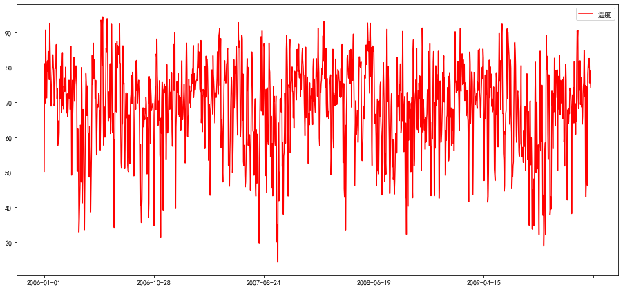
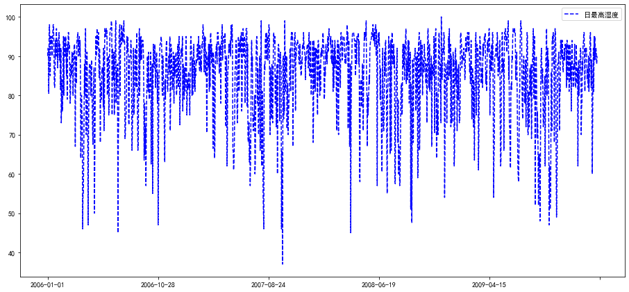
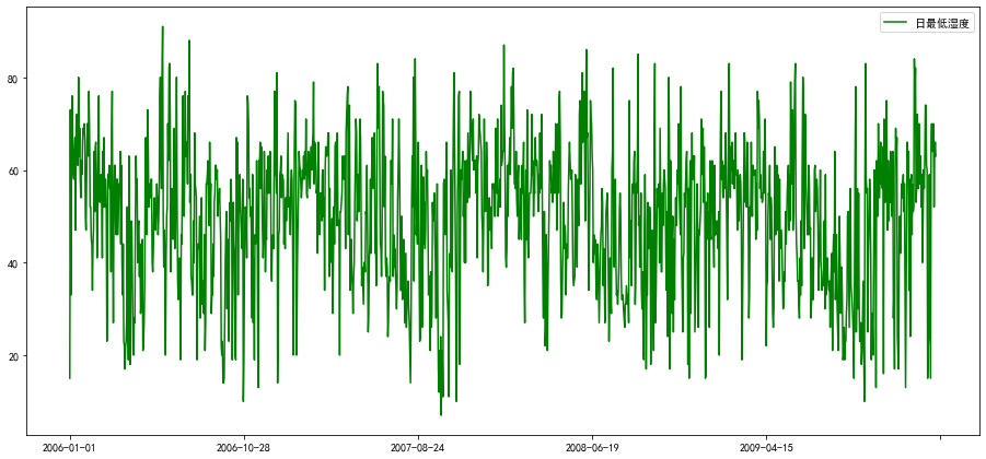
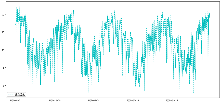
（2）绘制各气象信息的时间序列曲线

charts=datas["2006/01/01":"2010/02/01"]
charts.index=charts.index.map(lambda x:str(x)[:10])

# 创建一个画布
fig = plt.figure(figsize=(15.6,7.2))
# 在画布上添加一个子视图
ax = plt.subplot(111)
# 将x轴的刻度进行格式化
x_major_locator=MultipleLocator(300)      # 把x轴的刻度间隔设置为原来的2倍
ax.xaxis.set_major_locator(x_major_locator)  # 把x轴的主刻度设置为1的倍数
# 画折线
line1,=ax.plot(charts.index,charts['湿度'],'r-',label='湿度')  
plt.legend()

<matplotlib.legend.Legend at 0x7f056d061f98>

# 创建一个画布
fig = plt.figure(figsize=(15.6,7.2))
# 在画布上添加一个子视图
ax = plt.subplot(111)
# 将x轴的刻度进行格式化
x_major_locator=MultipleLocator(300)      # 把x轴的刻度间隔设置为原来的2倍
ax.xaxis.set_major_locator(x_major_locator)  # 把x轴的主刻度设置为1的倍数
# 画折线
line2,=ax.plot(charts.index,charts['日最高湿度'],'b--',label='日最高湿度')
plt.legend()

<matplotlib.legend.Legend at 0x7f06514f3908>

# 创建一个画布
fig = plt.figure(figsize=(15.6,7.2))
# 在画布上添加一个子视图
ax = plt.subplot(111)
# 将x轴的刻度进行格式化
x_major_locator=MultipleLocator(300)      # 把x轴的刻度间隔设置为原来的2倍
ax.xaxis.set_major_locator(x_major_locator)  # 把x轴的主刻度设置为1的倍数
# 画折线
line3,=ax.plot(charts.index,charts['日最低湿度'],'g-',label='日最低湿度')
plt.legend()

<matplotlib.legend.Legend at 0x7f056cf01a58>

# 创建一个画布
fig = plt.figure(figsize=(15.6,7.2))
# 在画布上添加一个子视图
ax = plt.subplot(111)
# 将x轴的刻度进行格式化
x_major_locator=MultipleLocator(300)      # 把x轴的刻度间隔设置为原来的2倍
ax.xaxis.set_major_locator(x_major_locator)  # 把x轴的主刻度设置为1的倍数
# 画折线
line4,=ax.plot(charts.index,charts['露点温度'],'c--',label='露点温度')
plt.legend()

<matplotlib.legend.Legend at 0x7f056ce78c88>

# 创建一个画布
fig = plt.figure(figsize=(15.6,7.2))
# 在画布上添加一个子视图
ax = plt.subplot(111)
# 将x轴的刻度进行格式化
x_major_locator=MultipleLocator(300)      # 把x轴的刻度间隔设置为原来的2倍
ax.xaxis.set_major_locator(x_major_locator)  # 把x轴的主刻度设置为1的倍数
# 画折线
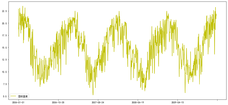
line5,=ax.plot(charts.index,charts['湿球温度'],'y-',label='湿球温度') 
plt.legend()

<matplotlib.legend.Legend at 0x7f056cdfb518>

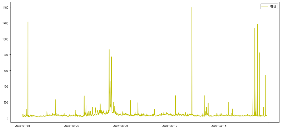
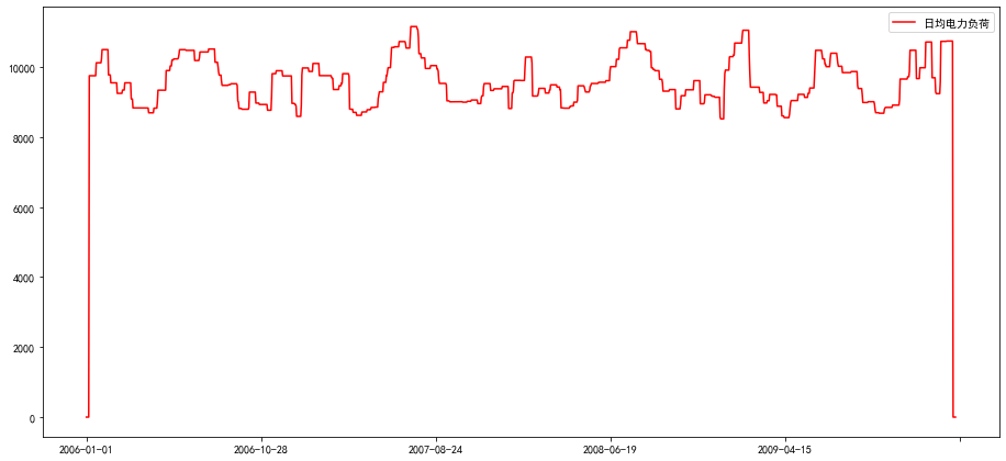
（3）绘制电价和电力负荷的时间序列曲线

chart=datas["2006/01/01":"2010/02/01"]
chart.index=chart.index.map(lambda x:str(x)[:10])

# 创建一个画布
fig = plt.figure(figsize=(15.6,7.2))
# 在画布上添加一个子视图
ax = plt.subplot(111)
#将x轴的刻度进行格式化
# ax.xaxis.set_major_formatter(mdate.DateFormatter('%Y/%m/%d'))
x_major_locator=MultipleLocator(300)      # 把x轴的刻度间隔设置为原来的2倍
ax.xaxis.set_major_locator(x_major_locator)  # 把x轴的主刻度设置为1的倍数
# 画折线
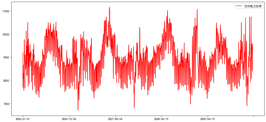
line1,=ax.plot(chart.index,chart['日均电力负荷'],'r-',label='日均电力负荷')  
plt.legend()

<matplotlib.legend.Legend at 0x7f056cd7e160>

# 创建一个画布
fig = plt.figure(figsize=(15.6,7.2))
# 在画布上添加一个子视图
ax = plt.subplot(111)
#将x轴的刻度进行格式化
# ax.xaxis.set_major_formatter(mdate.DateFormatter('%Y/%m/%d'))
x_major_locator=MultipleLocator(300)      # 把x轴的刻度间隔设置为原来的2倍
ax.xaxis.set_major_locator(x_major_locator)  # 把x轴的主刻度设置为1的倍数
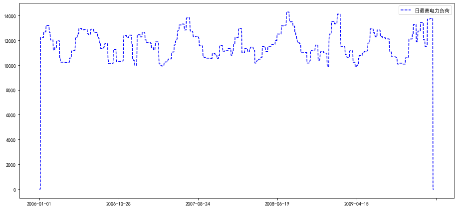
# 画折线
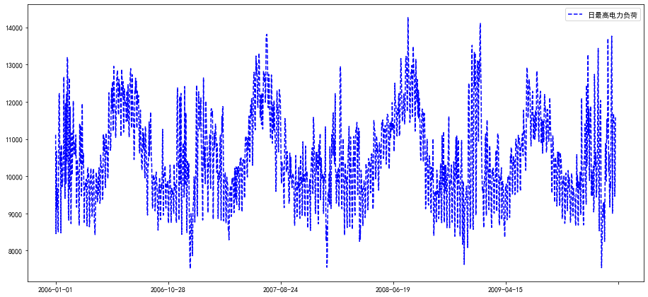
line2,=ax.plot(chart.index,chart['日最高电力负荷'],'b--',label='日最高电力负荷')
plt.legend()

<matplotlib.legend.Legend at 0x7f056cc59a58>

# 创建一个画布
fig = plt.figure(figsize=(15.6,7.2))
# 在画布上添加一个子视图
ax = plt.subplot(111)
#将x轴的刻度进行格式化
# ax.xaxis.set_major_formatter(mdate.DateFormatter('%Y/%m/%d'))
x_major_locator=MultipleLocator(300)      # 把x轴的刻度间隔设置为原来的2倍
ax.xaxis.set_major_locator(x_major_locator)  # 把x轴的主刻度设置为1的倍数
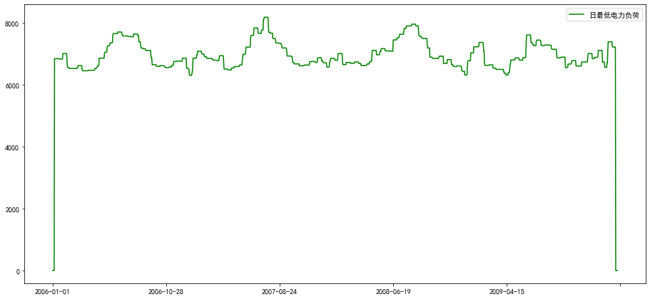
# 画折线
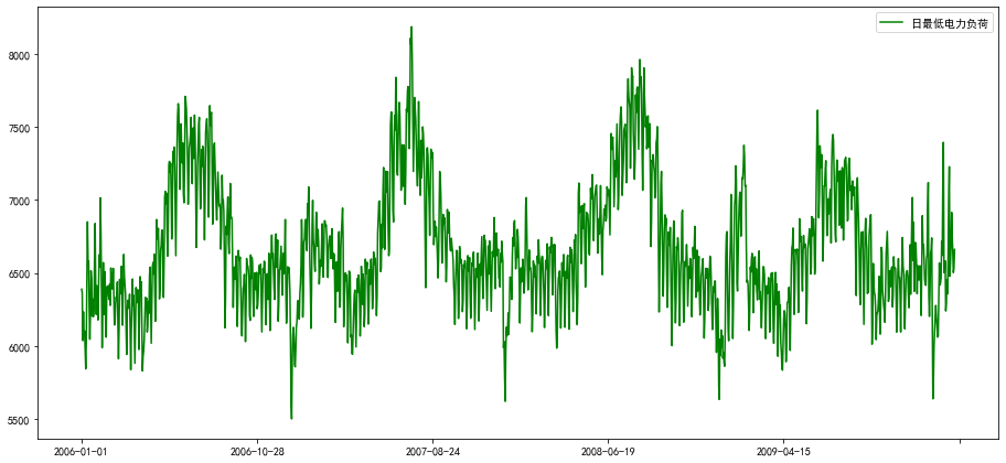
line3,=ax.plot(chart.index,chart['日最低电力负荷'],'g-',label='日最低电力负荷')  
plt.legend()

<matplotlib.legend.Legend at 0x7f056436af60>

chart=datas["2006/01/01":"2010/02/01"]
chart.index=chart.index.map(lambda x:str(x)[:10])

# 创建一个画布
fig = plt.figure(figsize=(15.6,7.2))
# 在画布上添加一个子视图
ax = plt.subplot(111)
# 将x轴的刻度进行格式化
# ax.xaxis.set_major_formatter(mdate.DateFormatter('%Y/%m/%d'))
x_major_locator=MultipleLocator(300)      # 把x轴的刻度间隔设置为原来的2倍
ax.xaxis.set_major_locator(x_major_locator)  # 把x轴的主刻度设置为1的倍数
# 画折线
line=ax.plot(chart.index,chart['电价'],'y-',label='电价')  
plt.legend()

<matplotlib.legend.Legend at 0x7f05642b8d68>

（4）编写中值滤波函数消除明显的噪音

def median_filter(data,sizes):
    filter_data=np.zeros_like(data)
    halfwindow=sizes
    for i in range (halfwindow,len(data)-halfwindow):
        window=data[i - halfwindow:i + halfwindow + 1]
        filter_data[i]=np.median(window)
    return filter_data

pd.options.mode.chained_assignment = None  # 默认模式
chart['干球温度']=median_filter(chart['干球温度'],5)
chart['日均电力负荷']=median_filter(chart['日均电力负荷'],5) 
chart['日最高电力负荷']=median_filter(chart['日最高电力负荷'],5) 
chart['日最低电力负荷']=median_filter(chart['日最低电力负荷'],5) 
chart['露点温度']=median_filter(chart['露点温度'],5) 

（5）绘制滤波后的时序曲线

# 创建一个画布
fig = plt.figure(figsize=(15.6,7.2))
# 在画布上添加一个子视图
ax = plt.subplot(111)
# 这里很重要  需要 将 x轴的刻度 进行格式化
# ax.xaxis.set_major_formatter(mdate.DateFormatter('%Y/%m/%d'))
x_major_locator=MultipleLocator(300)      # 把x轴的刻度间隔设置为原来的2倍
ax.xaxis.set_major_locator(x_major_locator)  # 把x轴的主刻度设置为1的倍数
# 画折线
line1,=ax.plot(chart.index,chart['日均电力负荷'],'r-',label='日均电力负荷')   
plt.legend()

<matplotlib.legend.Legend at 0x7f056402a7f0>

# 创建一个画布
fig = plt.figure(figsize=(15.6,7.2))
# 在画布上添加一个子视图
ax = plt.subplot(111)
# 这里很重要  需要 将 x轴的刻度 进行格式化
# ax.xaxis.set_major_formatter(mdate.DateFormatter('%Y/%m/%d'))
x_major_locator=MultipleLocator(300)      # 把x轴的刻度间隔设置为原来的2倍
ax.xaxis.set_major_locator(x_major_locator)  # 把x轴的主刻度设置为1的倍数
# 画折线
line2,=ax.plot(chart.index,chart['日最高电力负荷'],'b--',label='日最高电力负荷')  
plt.legend()

<matplotlib.legend.Legend at 0x7f056cdd9550>

# 创建一个画布
fig = plt.figure(figsize=(15.6,7.2))
# 在画布上添加一个子视图
ax = plt.subplot(111)
# 这里很重要  需要 将 x轴的刻度 进行格式化
# ax.xaxis.set_major_formatter(mdate.DateFormatter('%Y/%m/%d'))
x_major_locator=MultipleLocator(300)      # 把x轴的刻度间隔设置为原来的2倍
ax.xaxis.set_major_locator(x_major_locator)  # 把x轴的主刻度设置为1的倍数
# 画折线
line3,=ax.plot(chart.index,chart['日最低电力负荷'],'g-',label='日最低电力负荷')  
plt.legend()

<matplotlib.legend.Legend at 0x7f056cde05c0>

3.相关系数。求出各量与电力负荷之间的皮尔逊相关系数，选择相关系数绝对值前3高的属性作为特征属性，用于下一步进行模型训练。

#通常情况下通过以下取值范围判断变量的相关强度： 相关系数  0.8-1.0 极强相关 
#0.6-0.8  强相关  0.4-0.6     中等程度相关   0.2-0.4     弱相关  0.0-0.2     极弱相关或无相关
x=np.array([1,3,5])
y=np.array([1,3,4])
pc = pearsonr(x,y)
print("相关系数：",pc[0])
print("显著性水平：",pc[1])

相关系数： 0.9819805060619655
显著性水平： 0.1210377183236774

pccs = pearsonr(chart['湿度'],chart['日均电力负荷'])
print('湿度')
print("相关系数：",pccs[0])
print("显著性水平：",pccs[1])

湿度
相关系数： 0.008366098656828478
显著性水平： 0.7466985868452606

pccs = pearsonr(chart['干球温度'],chart['日均电力负荷'])
print('干球温度')
print("相关系数：",pccs[0])
print("显著性水平：",pccs[1])

干球温度
相关系数： 0.13553654698519382
显著性水平： 1.464772478253176e-07

pccs = pearsonr(chart['湿球温度'],chart['日均电力负荷'])
print('湿球温度')
print("相关系数：",pccs[0])
print("显著性水平：",pccs[1])

湿球温度
相关系数： -0.2234887241034933
显著性水平： 2.3520368633274703e-18

pccs = pearsonr(chart['露点温度'],chart['日均电力负荷'])
print('露点温度')
print("相关系数：",pccs[0])
print("显著性水平：",pccs[1])

露点温度
相关系数： 0.11306119537985258
显著性水平： 1.192249332196542e-05

pccs = pearsonr(chart['电价'],chart['日均电力负荷'])
print('电价')
print("相关系数：",pccs[0])
print("显著性水平：",pccs[1])

电价
相关系数： 0.12163330223784043
显著性水平： 2.436096002707336e-06

pccs = pearsonr(chart['日最高电力负荷'],chart['日均电力负荷'])
print('日最高电力负荷')
print("相关系数：",pccs[0])
print("显著性水平：",pccs[1])

日最高电力负荷
相关系数： 0.9766023264436509
显著性水平： 0.0

pccs = pearsonr(chart['日最低电力负荷'],chart['日均电力负荷'])
print('日最低电力负荷')
print("相关系数：",pccs[0])
print("显著性水平：",pccs[1])

日最低电力负荷
相关系数： 0.9390036936914716
显著性水平： 0.0

4.数据分析。使用上一步选择的3个特征属性作为输入属性，电力负荷作为输出属性，合理划分训练集与测试集比例，选择适合的参数，使用Sklearn建立决策树模型，并对模型进行测试。

（1）建立决策树模型

X=pd.concat([chart['湿球温度'],chart['干球温度'],chart['电价']],axis=1)
Y=chart['日均电力负荷']

# 划分测试与训练集
Xtrain,Xtest,Ytrain,Ytest=train_test_split(X,Y,test_size=0.1,random_state=420)
# 选择最优参数
tree_param={'criterion':['mse','friedman_mse','mae'],'max_depth':list(range(10))}

# GridSearchCV网格搜索，搜索的是参数，即在指定的参数范围内，按步长依次调整参数，利用调整的参数训练学习器，从所有的参数中找到在验证集上精度最高的参数，这其实是一个训练和比较的过程。k折交叉验证将所有数据集分成k份，不重复地每次取其中一份做测试集，
# 用其余k-1份做训练集训练模型，之后计算该模型在测试集上的得分,将k次的得分取平均得到最后的得分。
#实例化对象
grid=GridSearchCV(tree.DecisionTreeRegressor(),param_grid=tree_param,cv=3)

regressor = DecisionTreeRegressor(max_depth=5, min_samples_split=10)
grid = GridSearchCV(regressor, param_grid={'max_depth': [3, 5, 7], 'min_samples_split': [2, 5, 10]})
grid.fit(Xtrain, Ytrain)
#最优参数，最优分数
grid.best_params_,grid.best_score_
#建立回归树
dtr=tree.DecisionTreeRegressor(criterion='mae',max_depth =5)
#训练决策树
#预测训练结果
dtr.fit(Xtrain,Ytrain)
pred=dtr.predict(Xtest)

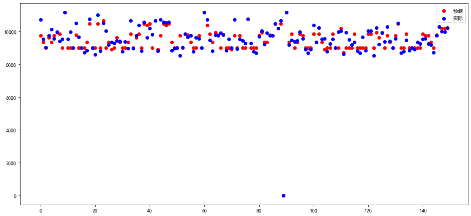
（2）绘制预测结果

fig=plt.figure(figsize=(15.6,7.2))
ax=fig.add_subplot(111)
s1=ax.scatter(range(len(pred)),pred,facecolors="red",label='预测')
s2=ax.scatter(range(len(Ytest)),Ytest,facecolors="blue",label='实际')
plt.legend()

<matplotlib.legend.Legend at 0x7f055ef94080>

实验总结：
自己总结一哈！