自编码器(Autoencoder)
AE
模型

import torch.nn as nn

class SimpleAE(nn.Module):
    def __init__(self):
        super().__init__()
        # 编码器:将输入数据压缩为更小的表示
        self.encoder = nn.Sequential(
            nn.Linear(28*28, 128),
            nn.ReLU(),
            nn.Linear(128, 32),
            nn.ReLU(),
            nn.Linear(32, 8)  # 压缩至 8 维
        )
        # 解码器:重建原始输入数据
        self.decoder = nn.Sequential(
            nn.Linear(8, 32),
            nn.ReLU(),
            nn.Linear(32, 128),
            nn.ReLU(),
            nn.Linear(128, 28*28),
            nn.Sigmoid()  # 输出在 0~1 之间
        )

    def forward(self, x):
        z = self.encoder(x)
        x = self.decoder(z)
        return x
训练
import torch as th
from torchvision import datasets, transforms
from torch.utils.data import DataLoader
import torch.optim as optim

# 超参数
batch_size = 128
epochs = 10

# 数据加载
train_dataset = datasets.MNIST('./data', train=True, download=True, transform=transforms.ToTensor())
train_loader = DataLoader(train_dataset, batch_size=batch_size, shuffle=True)

device = th.device("cuda" if th.cuda.is_available() else "cpu")
ae = SimpleAE().to(device)
criterion = nn.MSELoss()  # 使用均方误差损失
optimizer = optim.Adam(ae.parameters(), lr=1e-3)

ae.train()
for epoch in range(epochs):
    total_loss = 0
    for sample, _ in train_loader:
        input = sample.view(-1, 28*28).to(device)  # 展平图片为一维向量
        optimizer.zero_grad()
        output = ae(input)
        loss = criterion(output, input)
        loss.backward()
        optimizer.step()
        total_loss += loss.item()

    print(f'Epoch [{epoch+1}/{epochs}], Loss: {total_loss / batch_size:.4f}')
重建
import matplotlib.pyplot as plt
ae.eval()
# 加载测试集
test_dataset = datasets.MNIST('./data', train=False, download=True, transform=transforms.ToTensor())
test_loader = DataLoader(test_dataset, batch_size=4, shuffle=True)
# 取一批数据
data_iter = iter(test_loader)
sample, label = next(data_iter)
# 将图像输入 AE,得到重建图像
with th.no_grad():
input = sample.view(-1, 28*28).to(device)
output = ae(input)
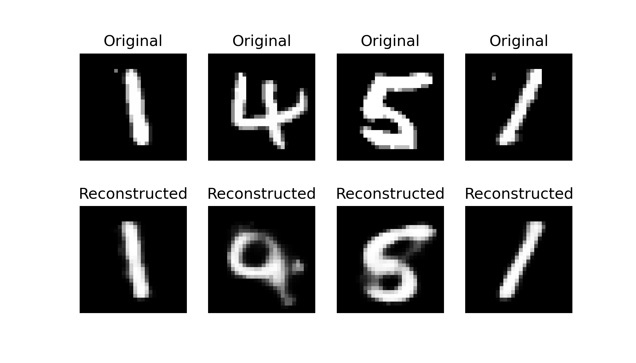
# 显示原始图像与重建图像对比
fig, axes = plt.subplots(2, 4, figsize=(7, 4))
recon = output.view(-1, 28, 28).cpu()
for i in range(4):
axes[0, i].imshow(sample[i].squeeze(), cmap='gray')
axes[0, i].axis('off')
axes[0, i].set_title("Original")
axes[1, i].imshow(recon[i].squeeze(), cmap='gray')
axes[1, i].axis('off')
axes[1, i].set_title("Reconstructed")
plt.show()
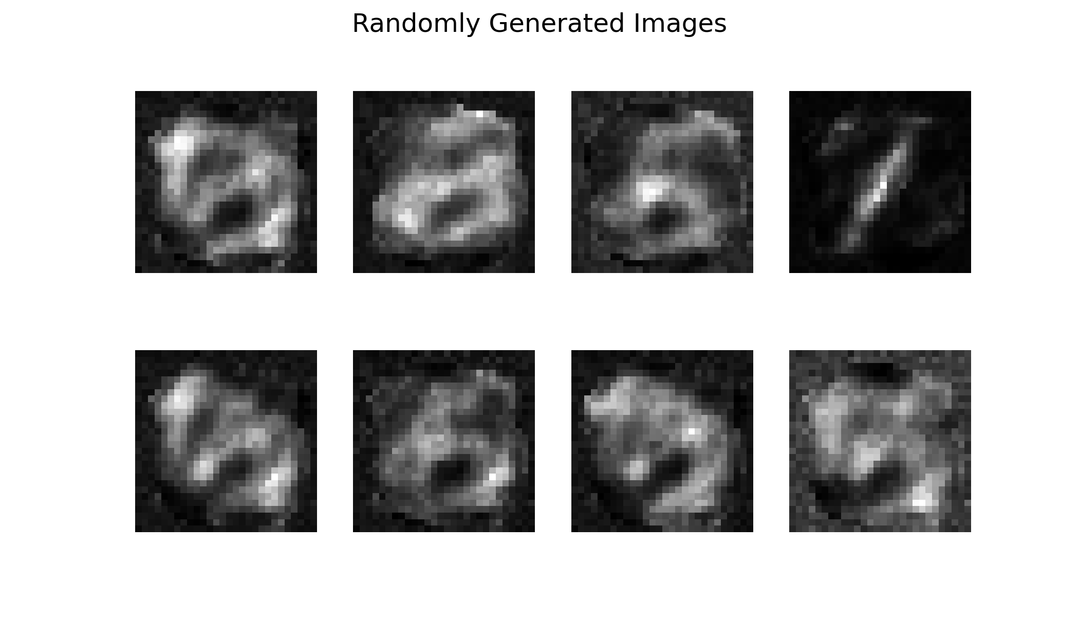
生成
with th.no_grad():
    z = th.randn(8, 8).to(device)  # 在隐变量空间随机采样(高斯分布)
    output = ae.decoder(z)

# 显示随机生成的图像
fig, axes = plt.subplots(2, 4, figsize=(7, 4))
sample = output.view(-1, 28, 28).cpu()

for i in range(8):
    axes[i // 4, i % 4].imshow(sample[i].squeeze(), cmap='gray')
    axes[i // 4, i % 4].axis('off')

plt.suptitle("Randomly Generated Images")
plt.show()
示例代码:SimpleAE | Kaggle
VAE
数学基础
AE 的目标是学到数据的低维表征,而 VAE 认为低维表征服从某个概率分布,并将目标改为学习概率分布的参数,然后从概率分布中采样得到低维表征。为了约束模型学习到的概率分布服从某具体分布,需要用到 KL 散度。为了从分布参数中采样得到样本,需要用到重参数化技巧。
KL 散度
KL 散度用于衡量两个概率分布之间的距离。
假设有两个正态分布 \(P(x)\) 和 \(Q(x)\),则 \(P\) 相对于 \(Q\) 的 KL 散度定义为:
重参数化
重参数化技巧将随机变量 \(z\sim\mathcal{N}(\mu,\sigma^2)\) 的采样过程分解为一个确定性函数和一个独立于参数的随机变量,使得梯度能够顺利地通过随机节点回传,从而实现有效的梯度估计。其标准形式为:
这样,虽然 \(z\) 看起来依然是随机的,但实际的随机性被“转移”到了 \(\epsilon\) 上,而 \(\mu\) 和 \(\sigma\) 部分则是一个确定性的可微函数。这样,在反向传播时,就可以直接计算关于 \(\mu\) 和 \(\sigma\) 的梯度,从而优化这些参数。
在 VAE 中,为方便优化,通常令模型直接输出 \(\mu\) 和 \(\log(\sigma^2)\) 而不是 \(\sigma\)(确保方差为正),于是会使用以下形式:
模型

import torch as th
import torch.nn as nn

def reparameterize(mu, logvar):
    std = th.exp(0.5 * logvar)
    eps = th.randn_like(std)
    return mu + std * eps

class SimpleVAE(nn.Module):
    def __init__(self):
        super().__init__()
        # 编码器
        self.encoder = nn.Sequential(
            nn.Linear(28*28, 128),
            nn.ReLU(),
            nn.Linear(128, 32),
            nn.ReLU(),
            nn.Linear(32, 16)
        )
        # 解码器
        self.decoder = nn.Sequential(
            nn.Linear(8, 32),
            nn.ReLU(),
            nn.Linear(32, 128),
            nn.ReLU(),
            nn.Linear(128, 28*28),
            nn.Sigmoid()
        )

    def forward(self, x):
        mu, logvar = self.encoder(x).chunk(2, dim=-1)
        z = reparameterize(mu, logvar)
        x = self.decoder(z)
        return x, mu, logvar
损失函数
VAE 的损失函数由两部分组成:
-
重建损失:衡量模型重构数据的能力,通常使用 MSE 或 BCE。(约束解码器还原图像)
-
KL 散度:衡量隐变量的后验分布与先验分布之间的差异。(约束编码器输出符合正态分布的 \(\mu\) 和 \(\log\sigma^2\))
如果令先验分布 \(p(z) \sim \mathcal{N}(0,1)\),后验分布 \(q_\phi(z \mid x) \sim \mathcal{N}(\mu,\sigma^2)\),则可得后验分布 \(q_\phi(z \mid x)\) 对先验分布 \(p(z)\) 的 KL 散度为:
\[D_{\mathrm{KL}}(q_\phi(z \mid x) \parallel p(z)) = -\frac{1}{2}\sum\left[1+\log\sigma^2-\mu^2-\sigma^2\right] \]
import torch.nn.functional as F

def criterion(recon, x, mu, logvar):
    MSE = F.mse_loss(recon, x, reduction='sum')                 # 重建损失
    KLD = -0.5 * th.sum(1 + logvar - mu.pow(2) - logvar.exp())  # KL 散度
    return MSE + KLD
训练
from torchvision import datasets, transforms
from torch.utils.data import DataLoader
import torch.optim as optim

# 超参数
batch_size = 128
epochs = 10

# 数据加载
train_dataset = datasets.MNIST('./data', train=True, download=True, transform=transforms.ToTensor())
train_loader = DataLoader(train_dataset, batch_size=batch_size, shuffle=True)

device = th.device("cuda" if th.cuda.is_available() else "cpu")
vae = SimpleVAE().to(device)
optimizer = optim.Adam(vae.parameters(), lr=1e-3)

vae.train()
for epoch in range(epochs):
    total_loss = 0
    for sample, _ in train_loader:
        input = sample.view(-1, 28*28).to(device)
        optimizer.zero_grad()
        output, mu, logvar = vae(input)
        loss = criterion(output, input, mu, logvar)
        loss.backward()
        optimizer.step()
        total_loss += loss.item()

    print(f'Epoch [{epoch+1}/{epochs}], Loss: {total_loss / batch_size:.4f}')
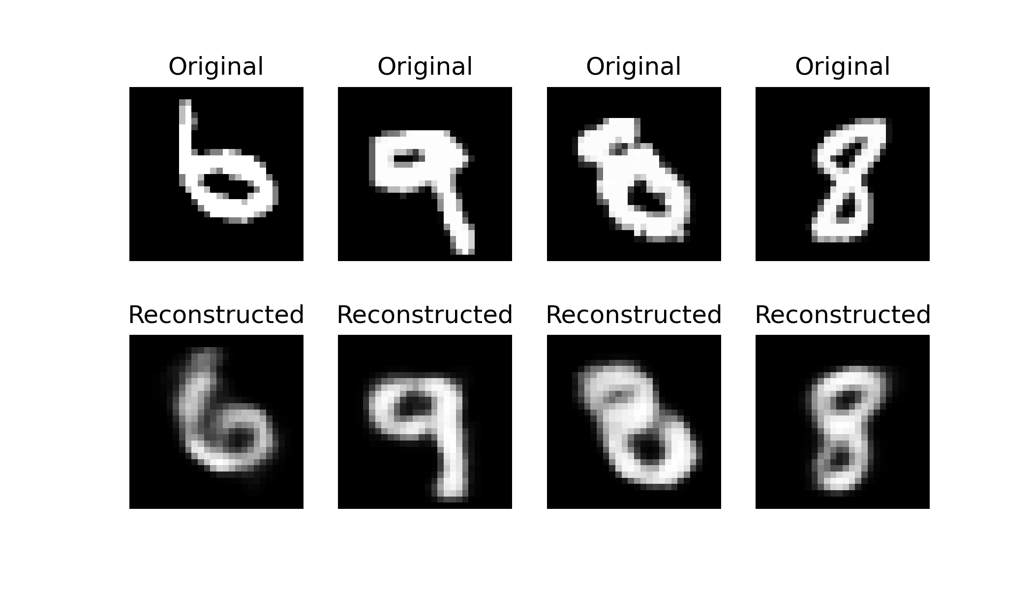
重建
测试已有图像重建效果(定性测试)
import matplotlib.pyplot as plt

vae.eval()

# 加载测试集
test_dataset = datasets.MNIST('./data', train=False, download=True, transform=transforms.ToTensor())
test_loader = DataLoader(test_dataset, batch_size=4, shuffle=True)

# 取一批数据
data_iter = iter(test_loader)
sample, label = next(data_iter)

# 将图像输入 VAE,得到重建图像
with th.no_grad():
    input = sample.view(-1, 28*28).to(device)
    output, _, _ = vae(input)

# 显示原始图像与重建图像对比
fig, axes = plt.subplots(2, 4, figsize=(7, 4))
recon = output.view(-1, 28, 28).cpu()

for i in range(4):
    axes[0, i].imshow(sample[i].squeeze(), cmap='gray')
    axes[0, i].axis('off')
    axes[0, i].set_title("Original")

    axes[1, i].imshow(recon[i].squeeze(), cmap='gray')
    axes[1, i].axis('off')
    axes[1, i].set_title("Reconstructed")

plt.show()
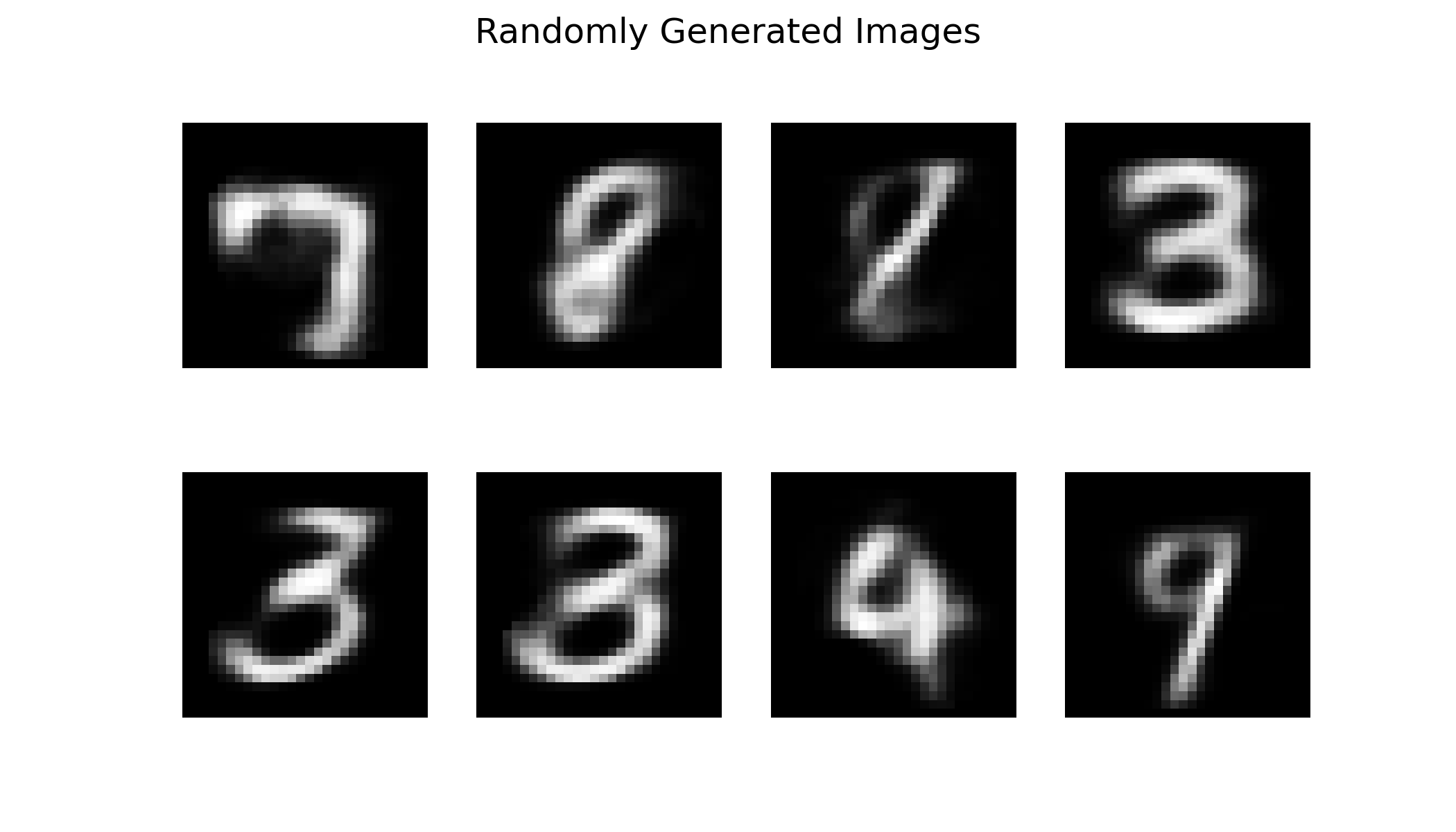
生成
随机采样生成新图像(从隐空间随机生成)
with th.no_grad():
    z = th.randn(8, 8).to(device)  # 在隐变量空间随机采样(高斯分布)
    output = vae.decoder(z)

# 显示随机生成的图像
fig, axes = plt.subplots(2, 4, figsize=(7, 4))
sample = output.view(-1, 28, 28).cpu()

for i in range(8):
    axes[i // 4, i % 4].imshow(sample[i].squeeze(), cmap='gray')
    axes[i // 4, i % 4].axis('off')

plt.suptitle("Randomly Generated Images")
plt.show()
示例代码:SimpleVAE | Kaggle
AE 与 VAE 的区别
| 特点 | AE | VAE |
|---|---|---|
| 网络结构 | 编码器 + 解码器,确定性 | 编码器 + 解码器,概率性 |
| 损失函数 | 重构误差 | 重构误差 + KL 散度 |
| 隐空间表示 | 不一定连续、规则 | 连续、规则 |
| 生成能力 | 弱 | 强(可随机生成) |
| 主要用途 | 降维、重建、去噪 | 数据生成、隐空间插值 |
MAE
Masked Autoencoder
模型
import torch.nn as nn

class SimpleMAE(nn.Module):
    def __init__(self):
        super().__init__()
        # 编码器
        self.encoder = nn.Sequential(
            nn.Linear(28*28, 128),
            nn.ReLU(),
            nn.Linear(128, 32),
            nn.ReLU(),
            nn.Linear(32, 8)
        )
        # 解码器
        self.decoder = nn.Sequential(
            nn.Linear(8, 32),
            nn.ReLU(),
            nn.Linear(32, 128),
            nn.ReLU(),
            nn.Linear(128, 28*28),
            nn.Sigmoid()
        )

    def forward(self, x, mask):
        x = x * mask
        z = self.encoder(x)
        x = self.decoder(z)
        return x
随机掩码
import torch as th

def random_mask(x, mask_ratio):
    """随机 mask 生成"""
    mask = th.bernoulli(th.full(x.shape, 1 - mask_ratio)).to(x.device)
    return mask
说明:
mask_ratio:决定遮挡比例。random_mask:生成和输入同维度的 0/1 mask 张量。- 损失只计算在被遮挡的区域(即 \(1-\text{mask}\) 部分)
训练
from torchvision import datasets, transforms
from torch.utils.data import DataLoader
import torch.optim as optim

# 超参数
mask_ratio = 0.8  # 遮挡 80% 的像素
batch_size = 128
epochs = 10

# 数据加载
train_dataset = datasets.MNIST(root='./data', train=True, download=True, transform=transforms.ToTensor())
train_loader = DataLoader(train_dataset, batch_size=batch_size, shuffle=True)

# 初始化模型与优化器
device = th.device('cuda' if th.cuda.is_available() else 'cpu')
mae = SimpleMAE().to(device)
criterion = nn.MSELoss()
optimizer = optim.Adam(mae.parameters(), lr=1e-3)

# 训练
for epoch in range(epochs):
    total_loss = 0
    for sample, _ in train_loader:
        input = sample.view(-1, 28*28).to(device)
        mask = random_mask(input, mask_ratio)
        optimizer.zero_grad()
        output = mae(input, mask)
        loss = criterion(output * (1 - mask), input * (1 - mask))  # 只计算遮挡区域的 loss
        loss.backward()
        optimizer.step()
        total_loss += loss.item()

    print(f'Epoch [{epoch+1}/{epochs}], Loss: {total_loss / batch_size:.4f}')
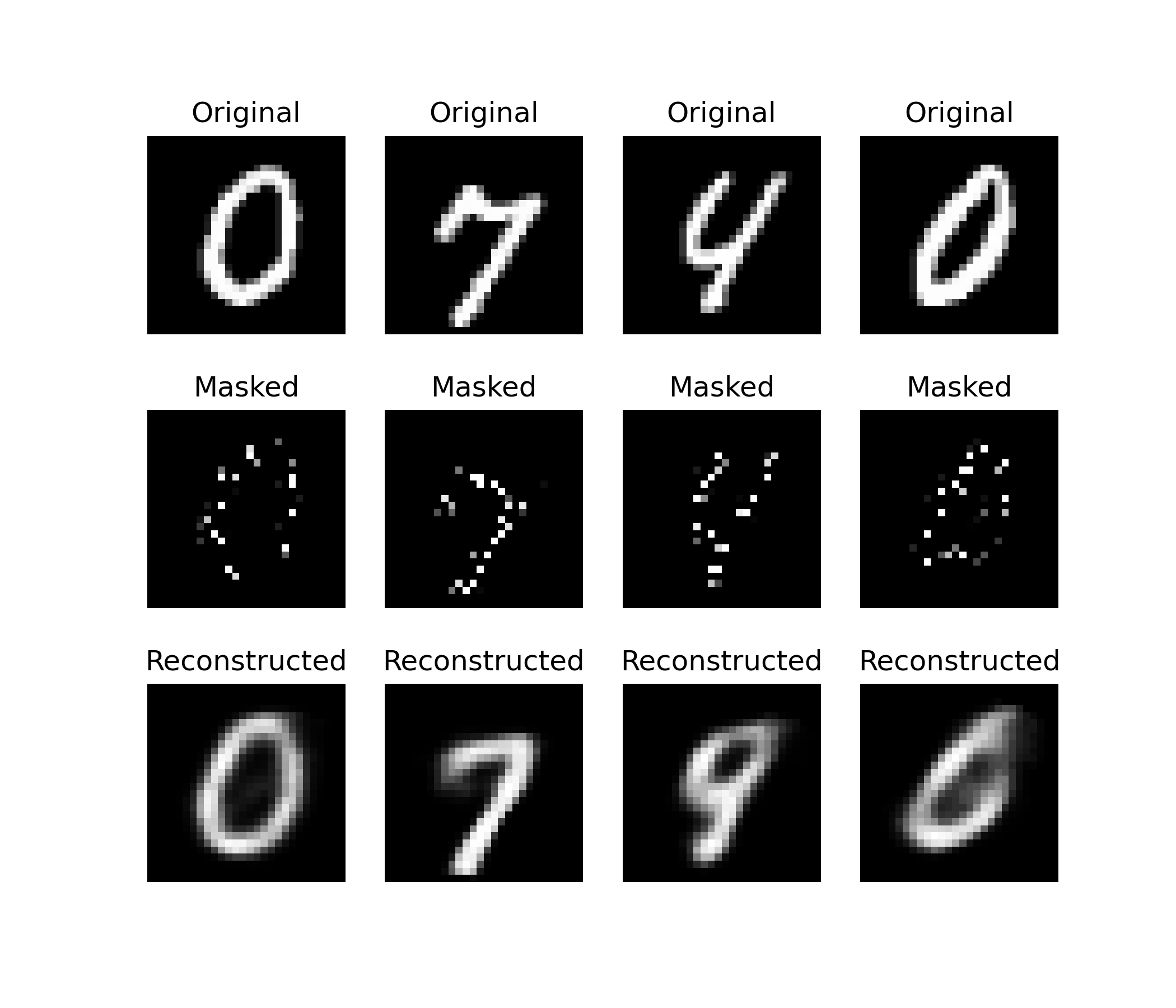
重建
import matplotlib.pyplot as plt

mae.eval()

test_dataset = datasets.MNIST('./data', train=False, download=True, transform=transforms.ToTensor())
test_loader = DataLoader(test_dataset, batch_size=4, shuffle=True)

data_iter = iter(test_loader)
sample, label = next(data_iter)

input = sample.view(-1, 28*28).to(device)
mask = random_mask(input, mask_ratio)

# 将图像输入 MAE,得到重建图像
with th.no_grad():
    output = mae(input, mask)

# 显示原始图像与重建图像对比
fig, axes = plt.subplots(3, 4, figsize=(7, 6))
masked_sample = (input * mask).view(-1, 28, 28).cpu()
recon = output.view(-1, 28, 28).cpu()

for i in range(4):
    axes[0, i].imshow(sample[i].squeeze(), cmap='gray')
    axes[0, i].axis('off')
    axes[0, i].set_title("Original")

    axes[1, i].imshow(masked_sample[i].squeeze(), cmap='gray')
    axes[1, i].axis('off')
    axes[1, i].set_title("Masked")

    axes[2, i].imshow(recon[i].squeeze(), cmap='gray')
    axes[2, i].axis('off')
    axes[2, i].set_title("Reconstructed")

plt.show()
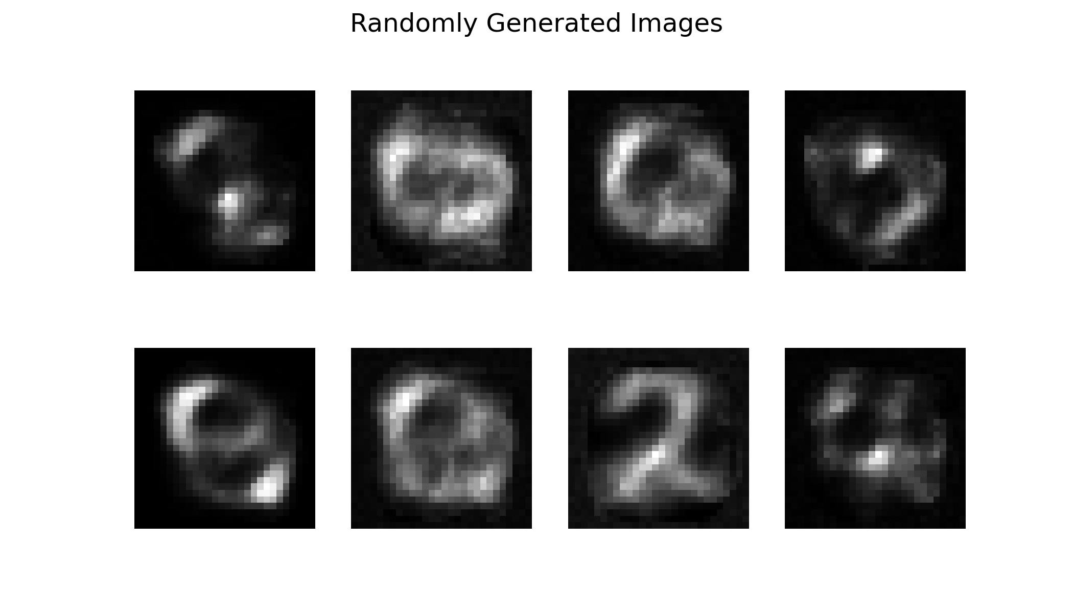
生成
with th.no_grad():
    z = th.randn(8, 8).to(device)  # 在隐变量空间随机采样(高斯分布)
    output = mae.decoder(z)

# 显示随机生成的图像
fig, axes = plt.subplots(2, 4, figsize=(7, 4))
sample = output.view(-1, 28, 28).cpu()

for i in range(8):
    axes[i // 4, i % 4].imshow(sample[i].squeeze(), cmap='gray')
    axes[i // 4, i % 4].axis('off')

plt.suptitle("Randomly Generated Images")
plt.show()
- 示例代码:SimpleMAE | Kaggle
- 论文:Masked Autoencoders Are Scalable Vision Learners | arXiv
- PyTorch 实现:facebookresearch/mae | GitHub
- 论文解读:MAE 论文逐段精读【论文精读】| BiliBili
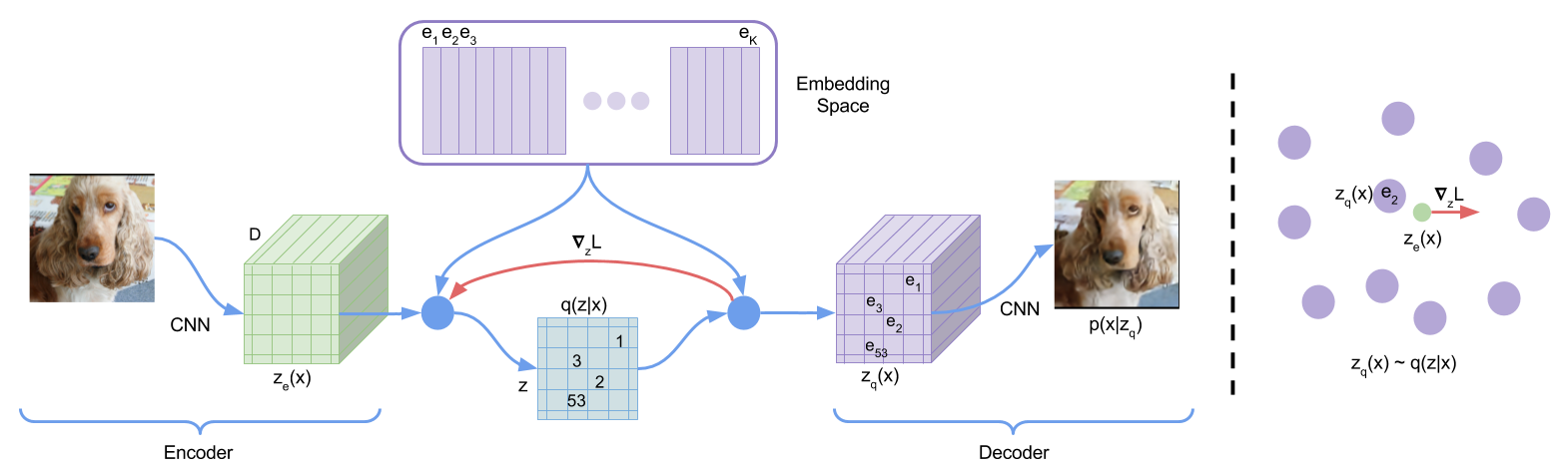
VQ-VAE
Vector Quantised-VAE,向量量化的 VAE。
将图像编码到离散潜空间,而不是连续潜空间。
- 其中 \(z_e(x)\) 是编码器输出
直通估计器:直接将解码器的输入(\(z_q(x)\))的梯度复制到编码器的输出(\(z_e(x)\))
- 其中 \(\operatorname{sg}\) 代表 stopgradient 运算符,该运算符在前向计算时定义为恒等映射,且其偏导数为零。
- 解码器仅优化第一个损失项,编码器优化第一个和最后一个损失项,嵌入向量由中间的损失项优化。

 浙公网安备 33010602011771号