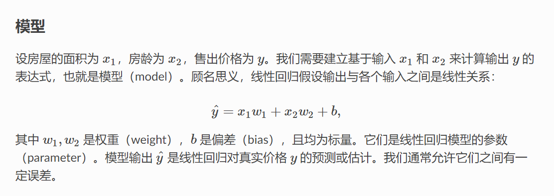
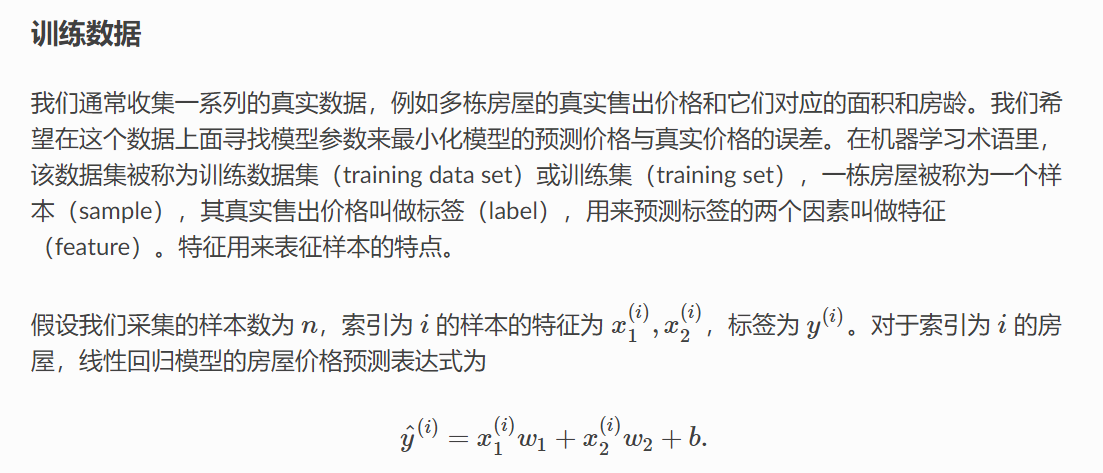
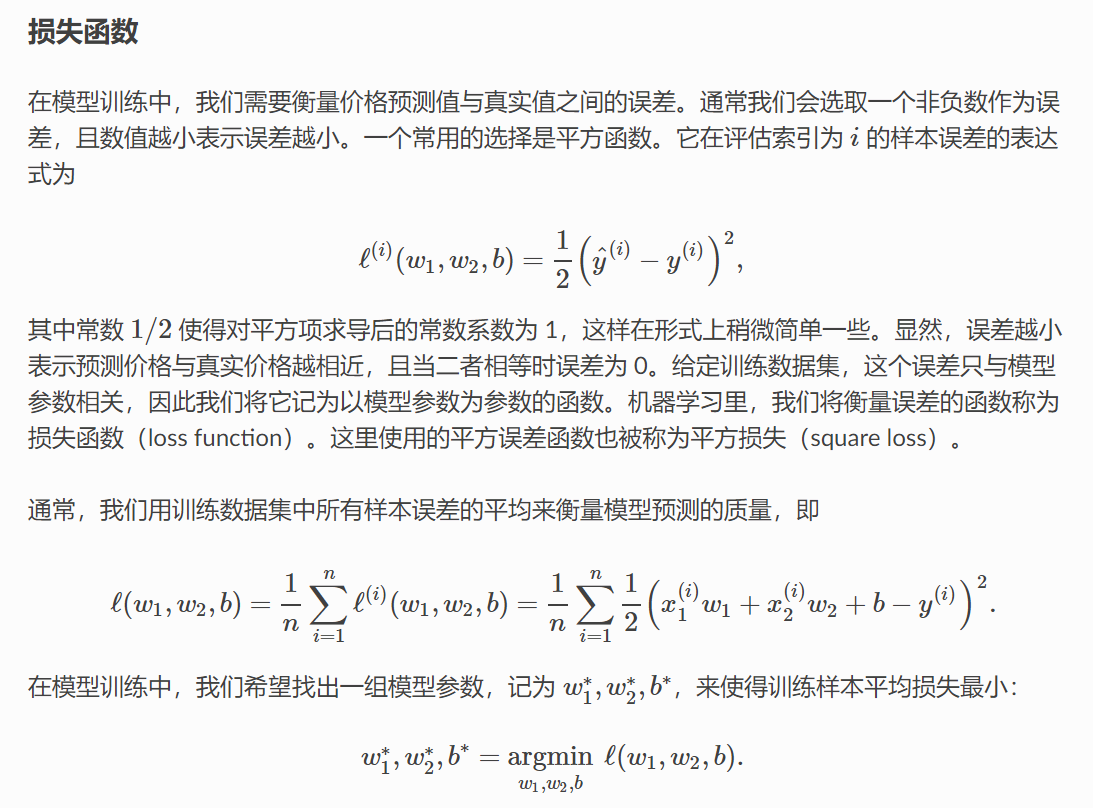
线性回归

 

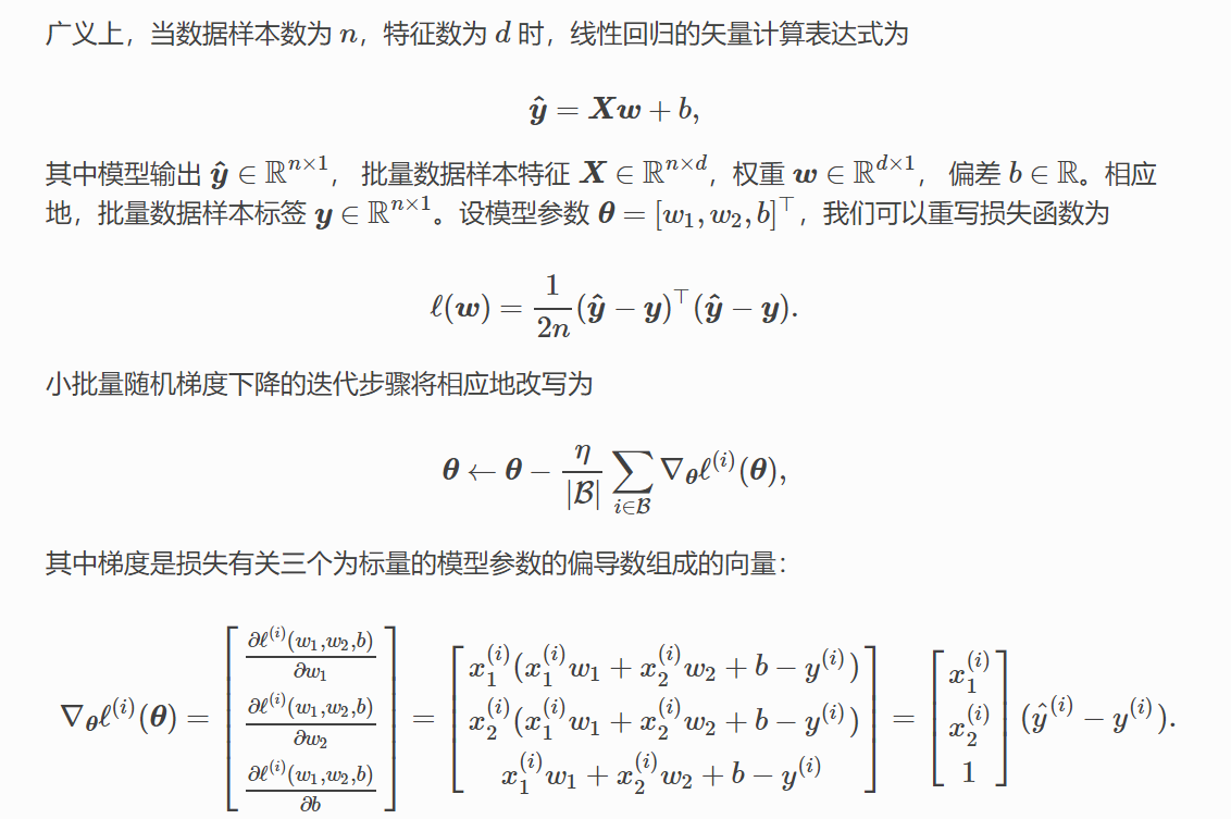
优化算法：小批量随机梯度下降

每次随机选择小样本，求小批量数据样本的平均损失函数的导数，修改模型参数。

 

 

矢量计算：

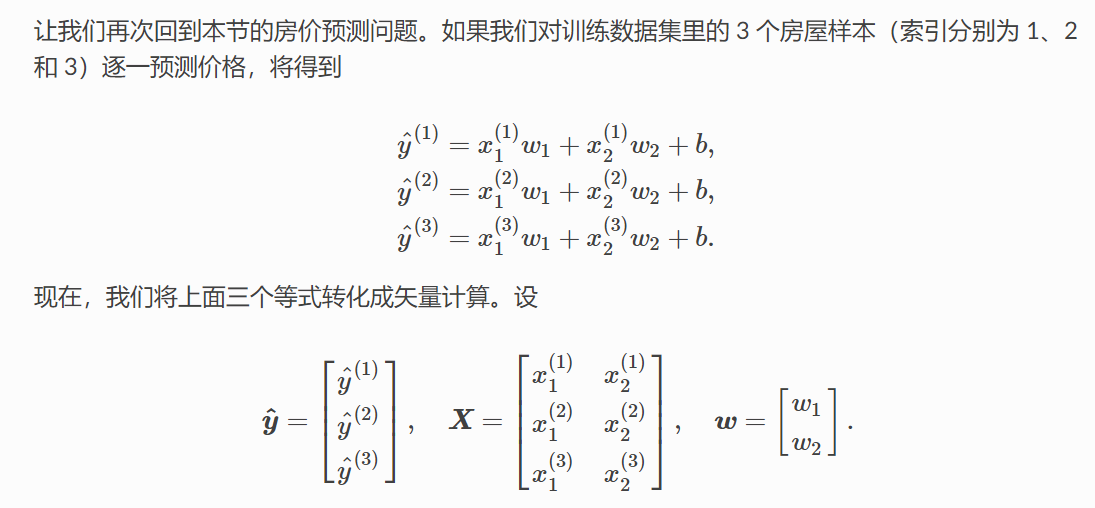
那么预测表达式为 y^ = XW + b

 

 

In [1]:

%matplotlib inline
from IPython import display
from matplotlib import pyplot as plt
from mxnet import autograd,nd
import random

In [2]:

num_inputs = 2
num_examples = 1000
true_w = [2,-3.4]
true_b = 4.2

features = nd.random.normal(scale=1,shape=(num_examples,num_inputs))

In [3]:

labels = true_w[0]*features[:,0] + true_w[1]*features[:,1] + true_b

In [4]:

labels += nd.random.normal(scale=0.01,shape=labels.shape)

In [5]:

features[0],labels[0]

Out[5]:

(
 [2.2122064 0.7740038]
 <NDArray 2 @cpu(0)>, 
 [6.000587]
 <NDArray 1 @cpu(0)>)

In [6]:

def use_svg_display():
    display.set_matplotlib_format('svg')

def set_figsize(figsize=(3.5,2.5)):
    use_svg_display()
    plt.rcParams['figure.figsize'] = figsize
    
set_figsize
plt.scatter(features[:,1].asnumpy(),labels.asnumpy(),1)

Out[6]:

<matplotlib.collections.PathCollection at 0x7fce5cd7bf50>

 

 

读取数据

In [7]:

def data_iter(batch_size, features, labels):
    num_examples = len(features)
    indices = list(range(num_examples))
    random.shuffle(indices)
    for i in range(0, num_examples, batch_size):
        j = nd.array(indices[i: min(i + batch_size, num_examples)])
        yield features.take(j), labels.take(j)

In [8]:

batch_size = 10

for X,y in data_iter(batch_size,features,labels):
    print(X,y)
    break

 

(
[[ 0.82885706  0.5436285 ]
 [-0.5273068   0.38621175]
 [ 0.5587636  -0.6481019 ]
 [-1.8886926   0.7965518 ]
 [ 0.63915503  0.89622647]
 [ 1.1829971  -0.03632846]
 [ 0.7806437   1.1585593 ]
 [ 0.5477088  -1.7779099 ]
 [ 0.5632628  -2.989     ]
 [-0.27784348  0.3698966 ]]
<NDArray 10x2 @cpu(0)>, 
[ 4.0100265  1.8428608  7.5078263 -2.284341   2.421783   6.6822963
  1.8219409 11.342728  15.501279   2.382981 ]
<NDArray 10 @cpu(0)>)

 

初始化模型参数¶

In [9]:

w = nd.random.normal(scale=0.01,shape=(num_inputs,1))
b = nd.zeros(shape=(1,))
w,b

Out[9]:

(
 [[-0.00939733]
  [-0.02246507]]
 <NDArray 2x1 @cpu(0)>, 
 [0.]
 <NDArray 1 @cpu(0)>)

 

w,b是迭代对象，创建他们的梯度

In [10]:

w.attach_grad()
b.attach_grad()

 

计算函数

In [11]:

def linreg(X, w, b):  # 本函数已保存在 gluonbook 包中方便以后使用。
    return nd.dot(X, w) + b

 

损失函数

In [12]:

def squared_loss(y_hat, y):  # 本函数已保存在 gluonbook 包中方便以后使用。
    return (y_hat - y.reshape(y_hat.shape)) ** 2 / 2

 

定义优化算法

In [13]:

def sgd(params, lr, batch_size):  # 本函数已保存在 gluonbook 包中方便以后使用。
    for param in params:
        param[:] = param - lr * param.grad / batch_size

 

训练模型¶

In [14]:

lr = 0.03
num_epochs = 3
net = linreg
loss = squared_loss

for epoch in range(num_epochs):  # 训练模型一共需要 num_epochs 个迭代周期。
    # 在一个迭代周期中，使用训练数据集中所有样本一次（假设样本数能够被批量大小整除）。
    # X 和 y 分别是小批量样本的特征和标签。
    for X, y in data_iter(batch_size, features, labels):
        with autograd.record():
            l = loss(net(X, w, b), y)  # l 是有关小批量 X 和 y 的损失。
        l.backward()  # 小批量的损失对模型参数求梯度。
        sgd([w, b], lr, batch_size)  # 使用小批量随机梯度下降迭代模型参数。
    train_l = loss(net(features, w, b), labels)
    print('epoch %d, loss %f' % (epoch + 1, train_l.mean().asnumpy()))
    

 

epoch 1, loss 0.040647
epoch 2, loss 0.000167
epoch 3, loss 0.000050

In [15]:

true_w,w

Out[15]:

([2, -3.4], 
 [[ 1.9999753]
  [-3.3995476]]
 <NDArray 2x1 @cpu(0)>)

In [16]:

true_b,b

Out[16]:

(4.2, 
 [4.1996946]
 <NDArray 1 @cpu(0)>)