机器学习—降维-特征选择6-2（包装法）

使用包装法对糖尿病数据集降维（递归特征消除法）

主要步骤流程：

• 1. 导入包
• 2. 导入数据集
• 3. 数据预处理
  • 3.1 检测缺失值
  • 3.2 生成自变量和因变量
  • 3.3 拆分训练集和测试集
  • 3.4 特征缩放
• 4. 使用递归特征消除法降维
• 5. 得到降维后的自变量

 

数据集链接：https://www.cnblogs.com/ojbtospark/p/16014512.html

 

1. 导入包

In [2]:

# 导入包
import numpy as np
import pandas as pd
import matplotlib.pyplot as plt

 

2. 导入数据集

In [3]:

# 导入数据集
dataset = pd.read_csv('pima-indians-diabetes.csv')
dataset

Out[3]:

	preg	plas	pres	skin	test	mass	pedi	age	class
0	6	148	72	35	0	33.6	0.627	50	1
1	1	85	66	29	0	26.6	0.351	31	0
2	8	183	64	0	0	23.3	0.672	32	1
3	1	89	66	23	94	28.1	0.167	21	0
4	0	137	40	35	168	43.1	2.288	33	1
...	...	...	...	...	...	...	...	...	...
763	10	101	76	48	180	32.9	0.171	63	0
764	2	122	70	27	0	36.8	0.340	27	0
765	5	121	72	23	112	26.2	0.245	30	0
766	1	126	60	0	0	30.1	0.349	47	1
767	1	93	70	31	0	30.4	0.315	23	0

768 rows × 9 columns

 

3. 数据预处理

3.1 检测缺失值

In [4]:

# 检测缺失值
null_df = dataset.isnull().sum()
null_df

Out[4]:

preg     0
plas     0
pres     0
skin     0
test     0
mass     0
pedi     0
age      0
class    0
dtype: int64

3.2 生成自变量和因变量

In [5]:

# 生成自变量和因变量
X = dataset.iloc[:,0:8].values
y = dataset.iloc[:,8].values

3.3 拆分训练集和测试集

In [6]:

# 拆分训练集和测试集
from sklearn.model_selection import train_test_split
X_train, X_test, y_train, y_test = train_test_split(X, y, test_size = 0.2, random_state = 1)
print(X_train.shape)
print(X_test.shape)
print(y_train.shape)
print(y_test.shape)

(614, 8)
(154, 8)
(614,)
(154,)

3.4 特征缩放

In [7]:

# 特征缩放
from sklearn.preprocessing import StandardScaler
sc_X = StandardScaler()
X_train = sc_X.fit_transform(X_train)
X_test = sc_X.transform(X_test)

 

4. 使用递归特征消除法降维

In [8]:

# 建立逻辑回归模型
from sklearn.linear_model import LogisticRegression
model = LogisticRegression()

In [9]:

# 递归特征消除法
from sklearn.feature_selection import RFECV
rfecv = RFECV(estimator = model, min_features_to_select = 1, cv=5, verbose=1, step=1, scoring='accuracy')
rfecv = rfecv.fit(X_train, y_train)

Fitting estimator with 8 features.
Fitting estimator with 7 features.
Fitting estimator with 6 features.
Fitting estimator with 5 features.
Fitting estimator with 4 features.
Fitting estimator with 3 features.
Fitting estimator with 2 features.
Fitting estimator with 8 features.
Fitting estimator with 7 features.
Fitting estimator with 6 features.
Fitting estimator with 5 features.
Fitting estimator with 4 features.
Fitting estimator with 3 features.
Fitting estimator with 2 features.
Fitting estimator with 8 features.
Fitting estimator with 7 features.
Fitting estimator with 6 features.
Fitting estimator with 5 features.
Fitting estimator with 4 features.
Fitting estimator with 3 features.
Fitting estimator with 2 features.
Fitting estimator with 8 features.
Fitting estimator with 7 features.
Fitting estimator with 6 features.
Fitting estimator with 5 features.
Fitting estimator with 4 features.
Fitting estimator with 3 features.
Fitting estimator with 2 features.
Fitting estimator with 8 features.
Fitting estimator with 7 features.
Fitting estimator with 6 features.
Fitting estimator with 5 features.
Fitting estimator with 4 features.
Fitting estimator with 3 features.
Fitting estimator with 2 features.
Fitting estimator with 8 features.
Fitting estimator with 7 features.
Fitting estimator with 6 features.

In [10]:

# 打印降维后的重要信息
print("应该选择的字段个数：%d" % rfecv.n_features_)

应该选择的字段个数：5

In [11]:

print("选择的字段索引是：%s" % rfecv.support_)

选择的字段索引是：[ True  True  True False False  True  True False]

In [12]:

print("字段排名是：%s" % rfecv.ranking_)

字段排名是：[1 1 1 4 3 1 1 2]

In [13]:

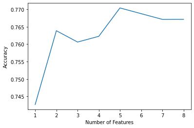
# 画出字段个数 VS 交叉验证分数
plt.figure()
plt.xlabel("Number of Features")
plt.ylabel("Accuracy")
plt.plot(range(1, len(rfecv.grid_scores_) + 1), rfecv.grid_scores_)
plt.show()

In [14]:

rfecv.grid_scores_

Out[14]:

array([0.74268959, 0.76385446, 0.76060243, 0.76224177, 0.77038518,
       0.76874583, 0.76710649, 0.76711982])

 

5. 得到降维后的自变量

In [15]:

# 得到降维后的自变量
features1 = rfecv.transform(X)
features1

Out[15]:

array([[  6.   , 148.   ,  72.   ,  33.6  ,   0.627],
       [  1.   ,  85.   ,  66.   ,  26.6  ,   0.351],
       [  8.   , 183.   ,  64.   ,  23.3  ,   0.672],
       ...,
       [  5.   , 121.   ,  72.   ,  26.2  ,   0.245],
       [  1.   , 126.   ,  60.   ,  30.1  ,   0.349],
       [  1.   ,  93.   ,  70.   ,  30.4  ,   0.315]])

In [16]:

# 得到降维后的自变量（验证）
features1 = X[:, [0,1,2,5,6]]
print(features1)

[[  6.    148.     72.     33.6     0.627]
 [  1.     85.     66.     26.6     0.351]
 [  8.    183.     64.     23.3     0.672]
 ...
 [  5.    121.     72.     26.2     0.245]
 [  1.    126.     60.     30.1     0.349]
 [  1.     93.     70.     30.4     0.315]]

 

结论：

features1 存储着降维后的自变量

 

 

 

 

 

 

 

​