机器学习—回归与分类4-2(随机森林算法)
使用随机森林预测德国人信贷风险
主要步骤流程:
- 1. 导入包
- 2. 导入数据集
- 3. 数据预处理
- 3.1 检测并处理缺失值
- 3.2 处理类别型变量
- 3.3 得到自变量和因变量
- 3.4 拆分训练集和测试集
- 3.5 特征缩放
- 4. 使用不同的参数构建随机森林模型
- 4.1 模型1:构建随机森林模型
- 4.1.1 构建模型
- 4.1.2 测试集做预测
- 4.1.3 评估模型性能
- 4.1.4 变量重要性排名
- 4.2 模型2:构建随机森林模型
- 4.3 模型3:构建随机森林模型
- 4.1 模型1:构建随机森林模型
1. 导入包
In [1]:
# 导入包
import numpy as np
import pandas as pd
2. 导入数据集
In [2]:
# 导入数据集
data = pd.read_csv("german_credit_data.csv")
data
Out[2]:
3. 数据预处理
3.1 检测并处理缺失值
In [3]:
# 检测缺失值
null_df = data.isnull().sum() # 检测缺失值
null_df
Out[3]:
In [4]:
# 处理Saving accounts 和 Checking account 这2个字段
for col in ['Saving accounts', 'Checking account']: # 处理缺失值
    data[col].fillna('none', inplace=True) # none说明这些人没有银行账户
In [5]:
# 检测缺失值
null_df = data.isnull().sum()
null_df
Out[5]:
3.2 处理类别型变量
In [6]:
# 处理Job字段
print(data.dtypes)
In [7]:
data['Job'] = data['Job'].astype('object')
In [8]:
# 处理类别型变量
data = pd.get_dummies(data, drop_first = True)
data
Out[8]:
3.3 得到自变量和因变量
In [9]:
# 得到自变量和因变量
y = data['Risk_good'].values
data = data.drop(['Risk_good'], axis = 1)
x = data.values
3.4 拆分训练集和测试集
In [10]:
# 拆分训练集和测试集
from sklearn.model_selection import train_test_split
x_train, x_test, y_train, y_test = train_test_split(x, y, test_size = 0.2, random_state = 1)
print(x_train.shape)
print(x_test.shape)
print(y_train.shape)
print(y_test.shape)
3.5 特征缩放
In [11]:
# 特征缩放
from sklearn.preprocessing import StandardScaler
sc_x = StandardScaler()
x_train = sc_x.fit_transform(x_train)
x_test = sc_x.transform(x_test)
4. 使用不同的参数构建随机森林模型
4.1 模型1:构建随机森林模型
4.1.1 构建模型
In [12]:
# 使用不同的参数构建随机森林模型
# 模型1:构建随机森林模型(max_depth=9, max_features='auto', min_samples_leaf=5, n_estimators=50)
from sklearn.ensemble import RandomForestClassifier
classifier = RandomForestClassifier(max_depth=9, max_features='auto', min_samples_leaf=5, n_estimators=50, random_state = 1)
classifier.fit(x_train, y_train)
Out[12]:
4.1.2 测试集做预测
In [13]:
# 在测试集做预测
y_pred = classifier.predict(x_test)
4.1.3 评估模型性能
In [14]:
# 评估模型性能
from sklearn.metrics import accuracy_score, confusion_matrix, classification_report
print(accuracy_score(y_test, y_pred))
In [15]:
print(confusion_matrix(y_test, y_pred))
In [16]:
print(classification_report(y_test, y_pred))
4.1.4 变量重要性排名
In [17]:
# 得到变量重要性排名
importance = classifier.feature_importances_
import matplotlib.pyplot as plt
plt.bar([x for x in range(len(importance))], importance)
plt.show()
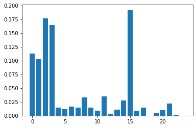
In [20]:
data.columns[2]
Out[20]:
通过变量重要性的柱状图可见,第0、1、2、3、15个自变量对因变量的影响较大。可以考虑做特征选择,进一步提升模型性能。特征选择在后面的章节会讲到。
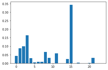
4.2 模型2:构建随机森林模型
In [21]:
# 模型2:构建随机森林模型(max_depth=3, max_features='auto', min_samples_leaf=50, n_estimators=100)
classifier = RandomForestClassifier(max_depth=3, max_features='auto', min_samples_leaf=50, n_estimators=100, random_state = 1)
classifier.fit(x_train, y_train)
Out[21]:
In [22]:
# 在测试集做预测
y_pred = classifier.predict(x_test)
In [23]:
# 评估模型性能
print(accuracy_score(y_test, y_pred))
In [24]:
print(confusion_matrix(y_test, y_pred))
In [25]:
print(classification_report(y_test, y_pred))
In [26]:
# 得到变量重要性排名
importance = classifier.feature_importances_
import matplotlib.pyplot as plt
plt.bar([x for x in range(len(importance))], importance)
plt.show()
4.3 模型3:构建随机森林模型
In [27]:
# 模型3:构建随机森林模型(max_depth=9, max_features=15, min_samples_leaf=5, n_estimators=25)
classifier = RandomForestClassifier(max_depth=9, max_features=15, min_samples_leaf=5, n_estimators=25, random_state = 1)
classifier.fit(x_train, y_train)
Out[27]:
In [28]:
# 在测试集做预测
y_pred = classifier.predict(x_test)
In [29]:
# 评估模型性能
print(accuracy_score(y_test, y_pred))
In [30]:
print(confusion_matrix(y_test, y_pred))
In [31]:
print(classification_report(y_test, y_pred))
In [32]:
# 得到变量重要性排名
importance = classifier.feature_importances_
import matplotlib.pyplot as plt
plt.bar([x for x in range(len(importance))], importance)
plt.show()
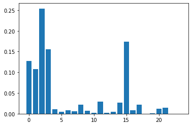
结论: 由上面3个模型可见,不同超参数对模型性能的影响不同

 浙公网安备 33010602011771号