主要步骤流程：

1. 导入包
2. 导入数据集
3. 数据预处理4. 构建逻辑回归模型
- 3.1 检测缺失值
- 3.2 生成自变量和因变量
- 3.3 查看样本是否均衡
- 3.4 将数据拆分成训练集和测试集
- 3.5 特征缩放
4.构建逻辑回归模型
5. 手工画出ROC曲线
6. 调用库画出ROC曲线
7. 得到AUC分数

数据集链接：https://www.cnblogs.com/ojbtospark/p/16006391.html

1. 导入包

In [1]:

# 导入包
import numpy as np
import pandas as pd
import matplotlib.pyplot as plt

2. 导入数据集

In [2]:

# 导入数据集
dataset = pd.read_csv('Social_Network_Ads.csv')
dataset

Out[2]:

	User ID	Gender	Age	EstimatedSalary	Purchased
0	15624510	Male	19	19000	0
1	15810944	Male	35	20000	0
2	15668575	Female	26	43000	0
3	15603246	Female	27	57000	0
4	15804002	Male	19	76000	0
...	...	...	...	...	...
395	15691863	Female	46	41000	1
396	15706071	Male	51	23000	1
397	15654296	Female	50	20000	1
398	15755018	Male	36	33000	0
399	15594041	Female	49	36000	1

400 rows × 5 columns

3. 数据预处理

3.1 检测缺失值

In [3]:

# 检测缺失值
null_df = dataset.isnull().sum()
null_df

Out[3]:

User ID            0
Gender             0
Age                0
EstimatedSalary    0
Purchased          0
dtype: int64

3.2 生成自变量和因变量

为了可视化分类效果，仅选取 Age 和 EstimatedSalary 这2个字段作为自变量

In [4]:

# 生成自变量和因变量
X = dataset.iloc[:, [2, 3]].values
y = dataset.iloc[:, 4].values

3.3 查看样本是否均衡

In [5]:

# 查看样本是否均衡
sample_0 = sum(dataset['Purchased']==0)
sample_1 = sum(dataset['Purchased']==1)
print('不买车的样本占总样本的%.2f' %(sample_0/(sample_0 + sample_1)))

不买车的样本占总样本的0.64

3.4 将数据拆分成训练集和测试集

In [6]:

# 将数据拆分成训练集和测试集
from sklearn.model_selection import train_test_split
X_train, X_test, y_train, y_test = train_test_split(X, y, test_size = 0.25, random_state = 0)
print(X_train.shape)
print(X_test.shape)
print(y_train.shape)
print(y_test.shape)

(300, 2)
(100, 2)
(300,)
(100,)

3.5 特征缩放

In [7]:

# 特征缩放
from sklearn.preprocessing import StandardScaler
sc = StandardScaler()
X_train = sc.fit_transform(X_train)
X_test = sc.transform(X_test)

4. 构建逻辑回归模型

In [8]:

# 构建逻辑回归模型并训练模型
from sklearn.linear_model import LogisticRegression
classifier = LogisticRegression(penalty='l2', C=1, class_weight='balanced', random_state = 0)
classifier.fit(X_train, y_train)

Out[8]:

LogisticRegression(C=1, class_weight='balanced', random_state=0)

In [9]:

# 预测测试集（得到预测结果）
y_pred = classifier.predict(X_test)
print(y_pred[:10])

[0 0 0 0 0 0 0 1 0 1]

In [10]:

# 预测测试集（得到概率）
y_pred_proba = classifier.predict_proba(X_test)[:,1]
print(y_pred_proba[:10])

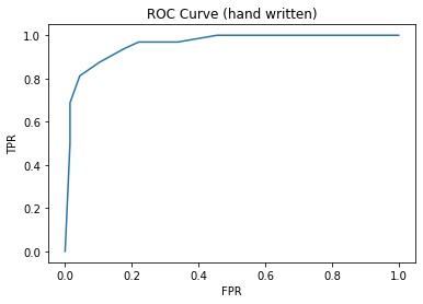
[0.15981512 0.23237193 0.27326099 0.12555781 0.13506028 0.00922329
 0.01852589 0.84130917 0.00685852 0.63294873]

5. 手工画出ROC曲线

In [11]:

# 手工画出ROC曲线
from sklearn.metrics import confusion_matrix
threshold_list = []
tpr_list = []
fpr_list = []
​
for i in range(11):
    threshold = i * 0.1 # threshold 分别为0、0.1、0.2、0.3、0.4、0.5、0.6、0.7、0.8、0.9、1
    new_y_pred_proba = []
    for j in y_pred_proba:
        if j >= threshold:
            new_y_pred_proba.append(1)
        else:
            new_y_pred_proba.append(0)
    cm = confusion_matrix(y_test, new_y_pred_proba) # 混淆矩阵
    tp = cm[1,1]
    fp = cm[0,1]
    fn = cm[1,0]
    tn = cm[0,0]
    tpr_value = tp/(tp+fn) # 计算tpr
    fpr_value = fp/(fp+tn) # 计算fpr
    threshold_list.append(threshold)
    tpr_list.append(tpr_value)
    fpr_list.append(fpr_value)
plt.figure()
plt.plot(fpr_list, tpr_list)
plt.xlabel('FPR')
plt.ylabel('TPR')
plt.title('ROC Curve (hand written)')
plt.show()

6. 调用库画出ROC曲线

In [12]:

# 求出ROC曲线用到的指标值
from sklearn.metrics import roc_curve
fpr, tpr, thresholds = roc_curve(y_test, y_pred_proba)

In [13]:

# 显示ROC曲线用到的指标值
roc_df = pd.DataFrame()
roc_df['fpr'] = fpr
roc_df['tpr'] = tpr
roc_df['thresholds'] = thresholds
roc_df

Out[13]:

	fpr	tpr	thresholds
0	0.000000	0.00000	1.998532
1	0.000000	0.03125	0.998532
2	0.000000	0.18750	0.991629
3	0.014706	0.18750	0.990037
4	0.014706	0.75000	0.677026
5	0.044118	0.75000	0.632949
6	0.044118	0.81250	0.602053
7	0.058824	0.81250	0.596452
8	0.058824	0.84375	0.563143
9	0.102941	0.84375	0.531246
10	0.102941	0.87500	0.521528
11	0.147059	0.87500	0.454756
12	0.147059	0.90625	0.429694
13	0.161765	0.90625	0.410702
14	0.161765	0.93750	0.402222
15	0.220588	0.93750	0.378048
16	0.220588	0.96875	0.346464
17	0.411765	0.96875	0.123208
18	0.411765	1.00000	0.118657
19	0.647059	1.00000	0.035503
20	0.676471	1.00000	0.034192
21	1.000000	1.00000	0.001963

In [14]:

# 画出ROC
plt.figure()
plt.plot(fpr, tpr)
plt.xlabel('FPR')
plt.ylabel('TPR')
plt.title('ROC Curve (call library)')
plt.show()

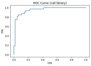
手工画出的ROC曲线和调用库画出的ROC曲线一致，说明我们对ROC的理解是正确的。

7. 得到AUC分数

In [15]:

# 得到AUC分数
from sklearn.metrics import roc_auc_score
auc_score = roc_auc_score(y_test, y_pred_proba)
print('AUC分数是：%.2f' %(auc_score))

AUC分数是：0.95

结论： AUC分数是0.95，说明模型性能非常好

一不小心就进橘子了

橘子种植园

机器学习—分类3-4（逻辑回归与ROC）