Mathametica_00_The Hertz' dipoles

Mathematica_00_画出赫兹偶极子的电场、磁场、坡印廷矢量的图像随时间的变化

Manipulate[
Pane[Module[{gg, inset1, inset2},
inset1 =
Inset[Graphics[
Text[Style["\!\(\*SubscriptBox[\(p\), \(0\)]\)", 20,
White]]], {0, 2.5}];
inset2 =
Inset[Graphics[
Text[Style[
Row[{Subscript[Style["p", Italic], 0], " sin \[Omega] ",
Style["t", Italic]}], 20, White]]], {0, 2.5}];
gg = Graphics[{Red, Rectangle[{-0.1, -0.2}, {0.1, 0.2}], White,
Thickness[0.01], Arrowheads[.05], Arrow[{{0, -0.2}, {0, 0.2}}]}];
If[f == "DC",
TableForm@{{Which[case == "Efield",
Show[ energydensity[
Table[W[Rv[[i]] Cos[\[Theta]v[[j]]],
Rv[[i]] Sin[\[Theta]v[[j]]]], {i, Length[Rv]}, {j,
Length[\[Theta]v]}]],
StreamPlot[Erz[r, z], {r, -3, 3}, {z, -3, 3},
StreamStyle -> Black],
gg, LabelStyle -> {FontSize -> 16}, Epilog -> inset1,
PlotLabel -> Style["electric field at DC condition", 16],
ImageSize -> {450, 380}],
case == "Mfield",
Graphics[{{huefunc[0], Rectangle[{-3, -3}, {3, 3}]},
{Red, Rectangle[{-0.1, -0.2}, {0.1, 0.2}], White,
Thickness[0.01], Arrowheads[.05],
Arrow[{{0, -0.2}, {0, 0.2}}]}},
PlotRange -> {{-3, 3}, {-3, 3}}, Axes -> None,
AspectRatio -> 1, Frame -> True,
LabelStyle -> {FontSize -> 16},
FrameLabel -> {Row[{Style["r", Italic], " (m)"}],
Row[{Style["z", Italic], " (m)"}], None, None},
LabelStyle -> {FontSize -> 16}, Epilog -> inset1,
PlotLabel -> Style["magnetic field at DC condition", 16],
ImageSize -> {450, 380}
],
case == "EMfield",
Show[
energydensity[
Table[W[Rv[[i]] Cos[\[Theta]v[[j]]],
Rv[[i]] Sin[\[Theta]v[[j]]]], {i, Length[Rv]}, {j,
Length[\[Theta]v]}]],
gg, LabelStyle -> {FontSize -> 16}, Epilog -> inset1,
PlotLabel -> Style["electric field at DC condition", 16],
ImageSize -> {450, 380}]], gscale[case]}},
\[Omega] = 2 \[Pi] 10^6 f ;
TableForm@{{Which[
case == "Efield",
Show[
energydensity[
Table[\[Epsilon]o/
2 (Norm[
Erz[Rv[[i]] Cos[\[Theta]v[[j]]],
Rv[[i]] Sin[\[Theta]v[[j]]], (
phase Degree)/\[Omega]]])^2, {i, Length[Rv]}, {j,
Length[\[Theta]v]}]],
StreamPlot[
Erz[r, z, (phase Degree)/\[Omega]], {r, -3, 3}, {z, -3, 3},
StreamStyle -> Black],
gg, LabelStyle -> {FontSize -> 16}, Epilog -> inset2,
PlotLabel ->
Style[Row[{"magnetic field at \[Omega] ",
Style["t", Italic], " = ", phase,
" degrees\nwavelength \[Lambda] = ",
NumberForm[(2 \[Pi] c)/\[Omega], {5, 3}], " m"}], 16],
ImageSize -> {450, 380}],
case == "Mfield",
Show[
energydensity[
Table[\[Mu]o/
2 (H\[Theta][Rv[[i]] Cos[\[Theta]v[[j]]],
Rv[[i]] Sin[\[Theta]v[[j]]], (
phase Degree)/\[Omega]])^2, {i, Length[Rv]}, {j,
Length[\[Theta]v]}]],
Graphics[
Table[If[H\[Theta][x, y, (phase Degree)/\[Omega]] > 0,
Join[dirplus[x, y], dirplus[x, -y], dirneg[-x, y],
dirneg[-x, -y]],

Join[dirneg[x, y], dirneg[x, -y], dirplus[-x, y],
dirplus[-x, -y]]], {x, 0.2, 3, 0.4}, {y, 0.2, 3, 0.4}]],
gg, LabelStyle -> {FontSize -> 16}, Epilog -> inset2,
PlotLabel ->
Style[Row[{"magnetic field at \[Omega] ",
Style["t", Italic], " = ", phase,
" degrees\nwavelength \[Lambda] = ",
NumberForm[(2 \[Pi] c)/\[Omega], {5, 3}], " m"}], 16],
ImageSize -> {450, 380}],
case == "EMfield",
Show[
energydensity[
Table[W[Rv[[i]] Cos[\[Theta]v[[j]]],
Rv[[i]] Sin[\[Theta]v[[j]]], (
phase Degree)/\[Omega]], {i, Length[Rv]}, {j,
Length[\[Theta]v]}]],
StreamPlot[
S[x, y, (phase Degree)/\[Omega]], {x, -3, 3}, {y, -3, 3},
StreamStyle -> Black],
gg, LabelStyle -> {FontSize -> 16}, Epilog -> inset2,
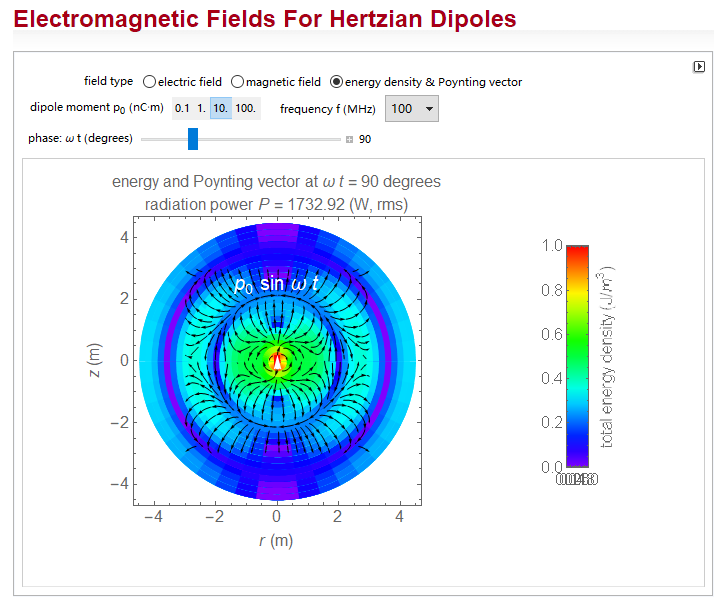
PlotLabel ->
Style[Row[{"energy and Poynting vector at \[Omega] ",
Style["t", Italic], " = ", phase,
" degrees\nradiation power ", Style["P", Italic],
" = ", (10^-18 \[Mu]o po^2 \[Omega]^4)/(12 \[Pi] c),
" (W, rms)"}], 16], ImageSize -> {450, 380}]],
gscale[case]}}]], ImageSize -> {650, 400}],

{{case, "Efield", "field type" }, {"Efield" -> "electric field",
"Mfield" -> "magnetic field",
"EMfield" -> "energy density & Poynting vector"},
ControlType -> RadioButtonBar, ControlPlacement -> Top},

Row[{
Control[{{po, 10.,
"dipole moment \!\(\*SubscriptBox[\(p\), \(0\)]\) (nC\
\[CenterDot]m)"}, {0.1, 1., 10., 100.}, ControlPlacement -> Top}],
Spacer[20],
Control[{{f, 100, "frequency f (MHz)"}, {"DC", 1, 3, 10, 30, 100,
300}, ControlPlacement -> Top}]}],

{{phase, 90, Row[{"phase: \[Omega] t (degrees)"}]}, 0, 360, 30,
Appearance -> "Labeled"},
TrackedSymbols :> {case, po, f, phase},
Initialization :> (
{\[Epsilon]o, \[Mu]o} = {8.854187818*10^-12, 4 \[Pi]*10^-7};
c = 1/Sqrt[\[Epsilon]o \[Mu]o];
huefunc[x_] := Hue[If[x > 1, 0., If[x < 0, 0.75, 0.75 (1 - x)]]];
Wr = 10^-3(*maximum enegy density to display*);
Erz[r_, z_] = (3*10^-9 po)/(
4 \[Pi] \[Epsilon]o) {(r z)/(r^2 + z^2)^(
5/2), -((r^2 - 2 z^2)/(r^2 + z^2)^(5/2))};
W[r_, z_] = (10^-18 po^2 (r^2 + 4 z^2))/(
32 \[Pi]^2 \[Epsilon]o (r^2 + z^2)^4);(*for dc condition*);
Erz[r_, z_, t_] :=
Im[(10^-9 po)/(
4 \[Pi] c^2 \[Epsilon]o) {-((
E^(I (t - Sqrt[r^2 + z^2]/c) \[Omega])
r z (-3 c^2 -
3 I c Sqrt[
r^2 + z^2] \[Omega] + (r^2 + z^2) \[Omega]^2))/ ((r^2 +
z^2)^(5/2)) ), (E^(
I (t - Sqrt[r^2 + z^2]/c) \[Omega]) (-c^2 (r^2 - 2 z^2) -
I c (r^2 - 2 z^2) Sqrt[r^2 + z^2] \[Omega] +
r^2 (r^2 + z^2) \[Omega]^2))/((r^2 + z^2)^(5/2))}];
H\[Theta][r_, z_, t_] :=
Im[-((10^-9 po)/(4 c \[Pi] )) (
E^(I (t - Sqrt[r^2 + z^2]/c) \[Omega])
r \[Omega] (-I c + Sqrt[r^2 + z^2] \[Omega]))/(r^2 + z^2)^(
3/2)];
W[r_, z_,
t_] := \[Epsilon]o/2 ( Norm[Erz[r, z, t]])^2 + \[Mu]o/
2 (H\[Theta][r, z, t])^2 ;
S[x_, z_,
t_] := {Im[-((
E^(I (t - Sqrt[x^2 + y^2]/c) \[Omega])
po x y (-3 c^2 -
3 I c Sqrt[x^2 + y^2] \[Omega] + (x^2 + y^2) \[Omega]^2))/(
4 c^2 \[Pi] (x^2 + y^2)^(5/2) \[Epsilon]o))]*
Im[-((E^(I (t - Sqrt[x^2 + y^2]/c) \[Omega])
po y \[Omega] (-I c + Sqrt[x^2 + y^2] \[Omega]))/(
4 c \[Pi] (x^2 + y^2)^(
3/2)))], -Im[(E^(I (t - Sqrt[x^2 + y^2]/c) \[Omega])
po (c^2 (2 x^2 - y^2) +
I c (2 x^2 - y^2) Sqrt[x^2 + y^2] \[Omega] +
y^2 (x^2 + y^2) \[Omega]^2))/(4 c^2 \[Pi] (x^2 + y^2)^(
5/2) \[Epsilon]o)]*
Im[-((E^(I (t - Sqrt[x^2 + y^2]/c) \[Omega])
po y \[Omega] (-I c + Sqrt[x^2 + y^2] \[Omega]))/(
4 c \[Pi] (x^2 + y^2)^(3/2)))]};
huefunc[x_] := Hue[If[x > 1, 0., If[x < 0, 0.75, 0.75 (1 - x)]]];
Wr = 10^-3;
Rv = Range[0.1, 4.5, 0.2]; \[Theta]v =
Range[\[Pi]/40, \[Pi]/2, \[Pi]/20];
energydensity[Wdata_] :=
Graphics[
Table[{huefunc[(6 + Log[10, Wdata[[Length[Rv] - i + 1, j]]/Wr])/
6], Disk[{0, 0},
Rv[[
Length[Rv] - i + 1]], {\[Theta]v[[j]] - \[Pi]/
40, \[Pi] - \[Theta]v[[j]] + \[Pi]/40}],
Disk[{0, 0},
Rv[[Length[Rv] - i + 1]], {-\[Pi] + \[Theta]v[[j]] - \[Pi]/
40, -\[Theta]v[[j]] + \[Pi]/40}]},
{i, Length[Rv]}, {j, Length[\[Theta]v]}] , Axes -> None,
AspectRatio -> 1, Frame -> True, LabelStyle -> {FontSize -> 16},
FrameLabel -> {Row[{Style["r", Italic], " (m)"}],
Row[{Style["z", Italic], " (m)"}], None, None}];
gscale[case_] :=
DensityPlot[y, {x, 0, 1}, {y, 0, 1},
PlotRange -> {{0, 1}, {0, 1}}, ColorFunctionScaling -> False,
AspectRatio -> 10, ColorFunction -> huefunc, Frame -> True,
FrameLabel ->
Which[case == "Efield", {None, "electric field (V/m)" , None,
"electric energy density (J/m\!\(\*SuperscriptBox[\(\\\ \), \
\(3\)]\))"},
case == "Mfield", {None, "magnetic field (A/m)" , None,
"magnetic energy density (J/\!\(\*SuperscriptBox[\(m\), \
\(3\)]\))"},
case == "EMfield", {None, Invisible["magnetic field (A/m)"] ,
None, "total energy density (J/\!\(\*SuperscriptBox[\(m\), \
\(3\)]\))"}],
FrameTicks -> {None, Which[
case == "Efield",
Table[{(6 + 2 k + Log[10, \[Epsilon]o/(2 Wr)])/6,
Superscript["10", ToString[k]]}, {k, 0, 4, 1}],
case == "Mfield",
Table[{(6 + 2 k + Log[10, \[Mu]o/(2 Wr)])/6,
ToString[1. 10^k]}, {k, -2, 2, 1}],
case == "EMfield", None],
None,
Table[{(6 + k - Log[10, Wr])/6,
Superscript["10", ToString[k]]}, {k, -11, -3, 1}]},
Axes -> None,
LabelStyle -> {FontSize -> 16},
ImageSize -> .9 Which[case == "Efield", 140, case == "Mfield",
137, case == "EMfield", 113.5]];
dirneg[x_, y_] := {White, Disk[{x, y}, 0.08], Blue,
Thickness[0.002], Circle[{x, y}, 0.08], Disk[{x, y}, 0.02]};
dirplus[x_, y_] := {White, Disk[{x, y}, 0.08], Blue,
Thickness[0.004], Circle[{x, y}, 0.08], Thickness[0.005],
Line[{{{x - 0.0566, y + 0.0566}, {x + 0.0566,
y - 0.0566}}, {{x - 0.0566, y - 0.0566}, {x + 0.0566,
y + 0.0566}}}]})]

原文链接，点击图片