
1 MATLAB常微分方程求解
1 找函数的解析解
1.1使用desolve函数,求解一阶微分方程
y1=dsolve('Dy==5');
y2=dsolve('Dy==x','x');
[y5,y6]=dsolve('Dx==y+x','Dy==2*x');
[y7,y8]=dsolve('Dx==y+x','Dy==2*x','x(0)==0','y(0)==1') ;
y9=dsolve('Dy==-2*y+2*x^2+2*x','y(0)==1','x') ;

%引号里的字符串都可以直接用变量代替
eqn10='Dy = y*x';
y10=dsolve(eqn10,'y(1)=1','x');

%画图方法
y10;
x = linspace(0,1,20);
z = eval(vectorize(y10));
plot(x,z)
结果
y1 = C1 + 5*t
y2 = x^2/2 + C2
y5 = C8*exp(2*t) - (C7*exp(-t))/2
y6 = C7*exp(-t) + C8*exp(2*t)
y7 = exp(2*t)/3 - exp(-t)/3
y8 = (2*exp(-t))/3 + exp(2*t)/3
y9 = exp(-2*x) + x^2
y10 = exp(-1/2)*exp(x^2/2)
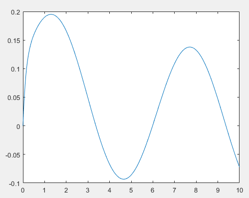
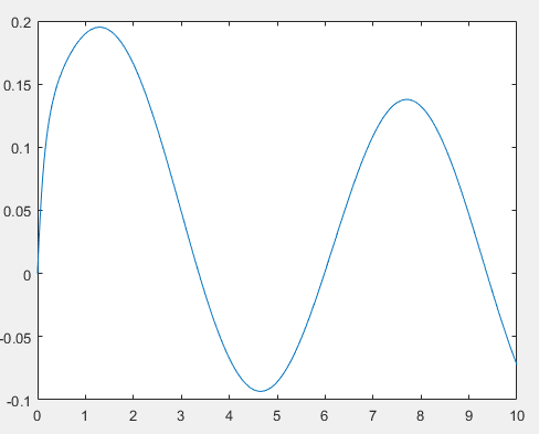
1.2使用desolve函数,求解二阶微分方程

eqn = 'D2y + 8*Dy + 2*y = cos(x)'; %D2y表示y''   Dy表示y'
inits = 'y(0) = 0,Dy(0) = 1';
y = dsolve(eqn,inits,'x');
x = linspace(0,10,300);
z = eval(vectorize(y));
plot(x,z);
结果
y = (14^(1/2)*exp(4*x - 14^(1/2)*x)*exp(x*(14^(1/2) - 4))*(sin(x) - cos(x)*(14^(1/2) - 4)))/(28*((14^(1/2) - 4)^2 + 1)) - (14^(1/2)*exp(4*x + 14^(1/2)*x)*exp(-x*(14^(1/2) + 4))*(sin(x) + cos(x)*(14^(1/2) + 4)))/(28*((14^(1/2) + 4)^2 + 1)) - (14^(1/2)*exp(-x*(14^(1/2) + 4))*(7*14^(1/2) + 27))/(28*(8*14^(1/2) + 31)) - (14^(1/2)*exp(x*(14^(1/2) - 4))*(393*14^(1/2) + 1531))/(28*(8*14^(1/2) - 31)*(8*14^(1/2) + 31)^2)
图像
1.3 使用desolve函数,求解方程组
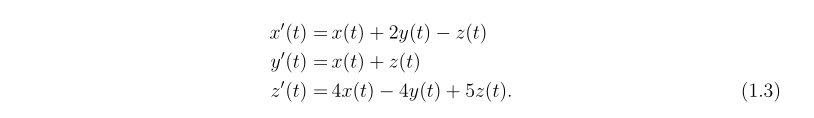
inits='x(0)=1,y(0)=2,z(0)=3';
[x,y,z]=dsolve('Dx=x+2*y-z','Dy=x+z','Dz=4*x-4*y+5*z',inits);
t = linspace(0,1,50);
xx = eval(vectorize(x))
yy = eval(vectorize(y))
zz = eval(vectorize(z))
plot(t,xx,'b',t,yy,'y',t,zz,'g')
解得:
x = 6*exp(2*t) - (5*exp(3*t))/2 - (5*exp(t))/2
y = (5*exp(3*t))/2 - 3*exp(2*t) + (5*exp(t))/2
z = 10*exp(3*t) - 12*exp(2*t) + 5*exp(t)
2 找函数的数值解
2.1 ode45函数 百度百科传送门 https://baike.baidu.com/item/ode45/6674723?fr=aladdin
2.2 inline函数解决一阶微分方程
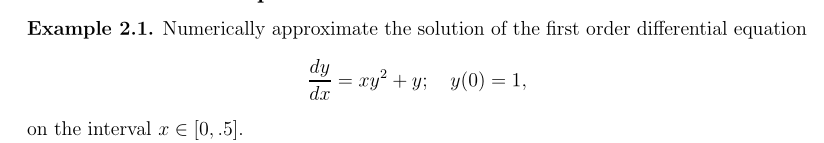
代码
f=inline('x*y^2+y');
[x,y]=ode45(f,[0 .5],1);
plot(x,y);
结果

增大步长(不设置步长的话,我也不知道初始步长是多少)
代码
xvalues=0:0.1:0.5
f=inline('x*y^2+y');
[x,y]=ode45(f,xvalues,1)
plot(x,y);
图像

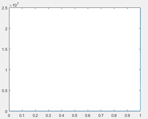
2.3 误差的控制
我们在使用ode45算法的时候,运算结果是有误差的。RelTol表示绝对误差AbsTol表示相对误差。ek表示k点的误差,yk表示k点的函数值。存在以下关系

当yk很大的时候,我们的误差就会很大,就会得到错误的结果。
实验案例如下。
代码
xvalues=0:0.001:1
f=inline('x*y^2+y');
[x,y]=ode45(f,xvalues,1)
plot(x,y);
图像

可以看出, 如果不控制RelTol的话,我们计算的最大值是
>> max(y)

ans =

   1.0033e+03
为了得到精确的结果,我们控制一下相对误差,让结果更加准确
代码
xvalues=0:0.001:1
options=odeset('RelTol',1e-10);
f=inline('x*y^2+y');
[x,y]=ode45(f,xvalues,1,options)
plot(x,y);
图像
查看最大值,这个值就比较准确了
>> max(y)

ans =

   2.4695e+07
2.4 把函数代码放到.m文件里。
还是这个式子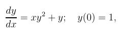
firstode.m
function yprime = firstode(x,y);
% FIRSTODE: Computes yprime = x*yˆ2+y
yprime = x*y^2 + y;
在使用ode45时候,我们要加一个 @ 符号就好了
test.m
xspan = [0,.5];
y0 = 1;
[x,y]=ode23(@firstode,xspan,y0);
plot(x,y)
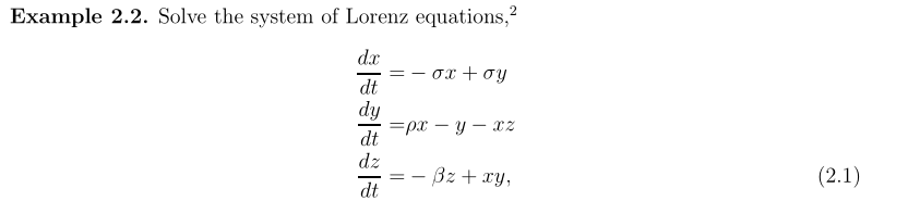
2.5 求解方程组

代码
lorenz.m
function xprime = lorenz(t,x);
%LORENZ: Computes the derivatives involved in solving the
%Lorenz equations.
sig=10;
beta=8/3;
rho=28;
xprime=[-sig*x(1) + sig*x(2); rho*x(1) - x(2) - x(1)*x(3); -beta*x(3) + x(1)*x(2)];
运行测试
test.m
x0=[-8 8 27];
tspan=[0,20];
[t,x]=ode45(@lorenz,tspan,x0)
plot(x(:,1),x(:,3)); %x(:,1)表示X  x(:,2)表示Y   x(:,3)表示Z
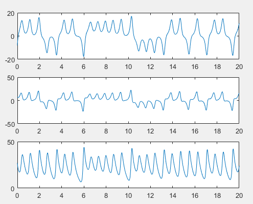
运行结果

test.m
 x0=[-8 8 27];
tspan=[0,20];
[t,x] = ode45(@lorenz,tspan,x0)
subplot(3,1,1);
plot(t,x(:,1));
subplot(3,1,2);
plot(t,x(:,2));
subplot(3,1,3);
plot(t,x(:,3));
运行结果
2.6 传递参数
lorenz1.m
function xprime = lorenz1(t,x,p);
%LORENZ: Computes the derivatives involved in solving the
%Lorenz equations.
sig=p(1); beta=p(2); rho=p(3);
xprime=[-sig*x(1) + sig*x(2); rho*x(1) - x(2) - x(1)*x(3); -beta*x(3) + x(1)*x(2)];
test.m
x0=[-8 8 27];
tspan=[0,20];
p=[10 8/3 28];
[t,x]=ode45(@lorenz1,tspan,x0,[],p);
plot(x(:,1),x(:,3))
应为传进去的参数和上次那个参数一模一样,所以这里就不贴图了。
2.7 二阶常微分方程求解

对于阶常微分方程的求解,可以通过增加变量个数的方式:Z=Y',然后增加方程个数,写成方程组的形式。
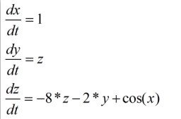
实现代码
F.m
function xprime = F(t,x);
%LORENZ: Computes the derivatives involved in solving the
%Lorenz equations.
xprime=[ 1 ; x(3) ; -8*x(3)-2*x(2)+cos( x(1) ) ];
test.m
x0=[0 0 1];
tspan=[0,10];
[t,x] = ode45(@F,tspan,x0)
plot(x(:,1),x(:,2)); %x(:,1)表示X  x(:,2)表示Y   x(:,3)表示Z
图像
3 拉普拉斯转换
3.1拉普拉斯变换
示例代码
>>syms t;
>>laplace(tˆ2)
3.2拉普拉斯逆变换
>>syms s;
>>ilaplace(1/(1+s))
4 边界值问题(我们不知道所有的初始值,但是知道边界值)
对于以下方程组:

代码
bc.m
function res=bc(L,R)
%BC: Evaluates the residue of the boundary condition
res=[L(1)-3;R(1)-10];  %L = 1    R= 10要写成这种形式。
bvpexample.m
function yprime = bvpexample(t,y)
%BVPEXAMPLE: Differential equation for boundary value
%problem example.
yprime=[y(2); -2*y(1)+3*y(2)];
test.m
sol=bvpinit(linspace(0,1,25),[0 1]);
sol=bvp4c(@bvpexample,@bc,sol);
plot( sol.x,sol.y(1,:) )
没学的部分1(资料不全,没Example3.1没办法先不学了)
没学的部分2 这一部分讲泰勒展开,高数老师没讲过,主要是一些数学原理,时间原因,先不学习。


 浙公网安备 33010602011771号