GAMES101

Introduction

the definition of CG

• computer graphics: the use of computer to synthesize and manipulate visual information

the application of CG

• video games
• movies
• animations
• design
• virtual reality
• illustration
• simulation
• GUI (Graphical User Interface)
• Typography（字体设计）

Why study computer graphics

• technical challenges
  • math of (perspective) projections, curves, surfaces
  • physics of lighting and shading
  • representing/operating shapes in 3D
  • animation/simulation
  • 3D graphics software programming and hardware
• CG is AWESOME

Course Topics

• Rasterization
  • Project geommetry primitives (3D triangles/polygons) onto the screen
  • break projected primitives into fragments(pixels)
  • gold standard in video games (real-time applications)
• Curves and Meshes
  • How to represent geometry in computer graphics
• Ray Tracing
  • shoot rays from the camera though each pixel
    • calculate intersection and shading
    • continue to bounce the rays till they hit light sources
  • gold standard in animation/movies (offline applications)
• Animation/Simulation
  • Key frame animation
  • mass-spring system
• NOT about:
  • using OpenGL/DirectX/Vulkan
  • 3D modeling using Maya/3DS MAX/Belnder, or VR/game development using Unity/Unreal Engine
  • computer vision/deep learing topics
• differences:
  • model \(\rightarrow\) image: CG (rendering)
  • model \(\rightarrow\) model: CG(modeling, simulation)
  • image \(\rightarrow\) image: CV(image processing)(not Computer Photography)
  • image \(\rightarrow\) model: CV

Course Logistic

• comprehensive but without hardware programming
• pace/contents subjecft to change
• use IDE
• textbook: tiger book

Basis

• CG dependencies:
  • mathematics: Algebra, calculus, statistics
  • physics: optics, mechanics
  • misc:
    • signal processing
    • numerical analysis
  • a bit of aesthetics

Linear Algebra

• vector: \(\vec a=(a_i)_n^T\) (column vector default)
  • vector addition
  • cartesian coordinate
  • dot(scalar) product
    • usage: same/opposite/vertical direction, length of vector
  • cross product
    • the judgement of right-handed system(RHS): \(\hat i \times \hat j=\hat k\)
    • usage: inside/outside, left/right
  • orthonormal coordinate frames:
    • \(\hat i \cdot \hat j=\hat j \cdot \hat k=\hat k \cdot \hat i=0\)
    • \(\hat i \times \hat j=\hat k\)
    • \(\vec p=(\vec p \cdot \hat i)\hat i+(\vec p \cdot \hat j)\hat j+(\vec p \cdot \hat k)\hat k\)
• matrix
  • matrix-matrix multiplication
    • associative and distributive
  • matrix-vector multiplication
  • transpose
  • vector multiplication in matrix form
    • dot product: \(\vec a \cdot \vec b=\vec a^T\vec b\)
    • cross product: \(\vec a \times \vec b=A^*\vec b\)
      • dual matrix: $$A^*=\left\lgroup\begin{matrix}
        0 & -z_a & y_a \
        z_a & 0 & -x_a \
        -y_a & x_a & 0 \
        \end{matrix}\right\rgroup$$

transformation

• why study transformation:
  • modeling: translation, rotation, scaling
  • viewing: (3D to 2D) projection
• categories of transformation:
  • Linear transformation: \(\vec x'=M\vec x\)
  • affine transform \(=\) linear transform \(+\) translation
  • inverse transform: \(M^{-1}\)
• Homogenous Coordinates:
  • 2D point: \((x,y,1)^T\)
    • \((x,y,a)^T=(\frac xa,\frac ya,1)^T\)
  • 2D vector: \((x,y,0)^T\)
  • why diff for point and vector:
    • vector \(+\) vector \(=\) vector
    • point \(-\) point \(=\) vector
    • point \(+\) vector \(=\) point
    • point \(+\) point \(=\) mid-point
• 2D transformations:
  • scale: \(S(s_x,s_y)=\left\lgroup\begin{matrix} s_x & 0 & 0\\ 0 & s_y & 0\\ 0 & 0 & 1\\ \end{matrix}\right\rgroup\)
    
    
  • reflection: \(R_x=\left\lgroup\begin{matrix} -1 & 0 & 0\\ 0 & 1 & 0\\ 0 & 0 & 1\\ \end{matrix}\right\rgroup,R_y=\left\lgroup\begin{matrix} 1 & 0 & 0\\ 0 & -1 & 0\\ 0 & 0 & 1\\ \end{matrix}\right\rgroup\)
    
    
  • shear: \(Sh(a)=\left\lgroup\begin{matrix} 1 & a & 0\\ 0 & 1 & 0\\ 0 & 0 & 1\\ \end{matrix}\right\rgroup\)
    
    
  • rotate: \(R(\theta)=\left\lgroup\begin{matrix} \cos\theta & -\sin\theta & 0\\ \sin\theta & \cos\theta & 0\\ 0 & 0 & 1\\ \end{matrix}\right\rgroup\)
    
    
  • translation: \(T(t_x,t_y)=\left\lgroup\begin{matrix} 1 & 0 & t_x\\ 0 & 1 & t_y\\ 0 & 0 & 1\\ \end{matrix}\right\rgroup\)
    
    
• composite transform: the multiplication of matrixes
  • formula representation: \(A_n(...A_2(A_1(\vec x)))=(A_n...A_2A_1)\vec x\)
  • one step forward \(\Leftrightarrow\) left multiplication of matrix
  • decomposing complex transformation: (take rotate around a given point c as example)
    1. translate center to origin
    2. rotate
    3. translate back
• 3D transformation: just add an axis based on 2D transformation (model transformation)
  • special: rotation: \(R_x(\theta)=\left\lgroup\begin{matrix} 1 & 0 & 0 & 0\\ 0 & \cos\theta & -\sin\theta & 0\\ o & \sin\theta & \cos\theta & 0\\ 0 & 0 & 0 & 1\\ \end{matrix}\right\rgroup, R_y(\theta)=\left\lgroup\begin{matrix} \cos\theta & 0 & \sin\theta & 0\\ 0 & 1 & 0 & 0\\ -\sin\theta & 0 & \cos\theta & 0\\ 0 & 0 & 0 & 1\\ \end{matrix}\right\rgroup,R_z(\theta)=\left\lgroup\begin{matrix} \cos\theta & -\sin\theta & 0 & 0\\ \sin\theta & \cos\theta & 0 & 0\\ 0 & 0 & 1 & 0\\ 0 & 0 & 0 & 1\\ \end{matrix}\right\rgroup\)
    
    
    • \(R_{xyz}(\alpha,\beta\gamma)=R_x(\alpha)R_y(\beta)R_z(\gamma)\)
    • \(R(\hat n,\alpha)=\cos\alpha I+(1-\cos\alpha)\hat n\hat n^T+\sin\alpha N\)
      • \(N=\left\lgroup\begin{matrix}0 & -n_z & n_y & 0\\n_z & 0 & -n_x & 0\\-n_y & n_x & 0 & 0\\0 & 0 & 0 & 1\\\end{matrix}\right\rgroup\)
• viewing transformation:
  • steps:
    1. find a good place and arrange people (model transformation)
    2. find a good "angle" to put the camera (view transformation)
    3. cheese! (projection transformation)
  • view/camera transformation
    • basic defs:
      • position: \(\vec e\)
      • look-at/gaze direction: \(\hat g\)
      • up direction: \(\hat t\)
    • key observation: If the camera and all objects move together, the photo will be the same \(\Rightarrow\) put camera at \((0,0)\) (the thing view transformation do)
    • steps:
      • translate \(\vec e\) to origin
      • rotate \(\hat g\) to \(-\hat k\)
      • rotate \(\hat t\) to \(\hat j\)
      • rotate \(\hat g \times \hat t\) to \(\hat i\)
    • representation: \(M_{view}=R_{view}T_{view}\)
      
      
      • \(T_{view}=\left\lgroup\begin{matrix} 1 & 0 & 0 & -x_e\\ 0 & 1 & 0 & -y_e\\ 0 & 0 & 1 & -z_e\\ 0 & 0 & 0 & 1\\ \end{matrix}\right\rgroup\)
        
        
      • \(R^{-1}_{view}=\left\lgroup\begin{matrix} x_{\hat g \times \hat t} & x_t & x_{-g} & 0\\ y_{\hat g \times \hat t} & y_t & y_{-g} & 0\\ z_{\hat g \times \hat t} & z_t & z_{-g} & 0\\ 0 & 0 & 0 & 1\\ \end{matrix}\right\rgroup \Rightarrow R_{view}=\left\lgroup\begin{matrix} x_{\hat g \times \hat t} & y_{\hat g \times \hat t} & z_{\hat g \times \hat t} & 0\\ x_t & y_t & z_t & 0\\ x_{-g} & y_{-g} & z_{-g} & 0\\ 0 & 0 & 0 & 1\\ \end{matrix}\right\rgroup\)
        
        
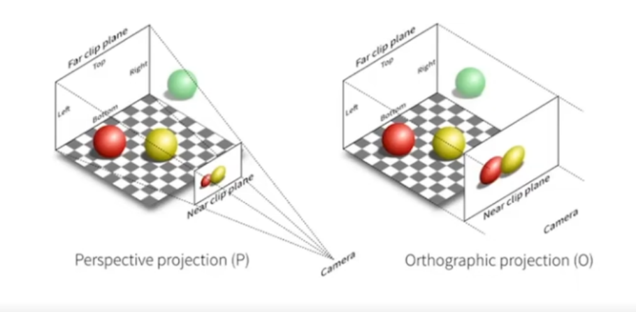
  • projection transformation
    • orthographic projection
      • basic defs:
        • cuboid: \([l,r] \times [b,t] \times [f,n]\)
        • "canonical" cube: \([-1,1]^3\)
      • a way to get orthographic projection:
        1. camera located at origin, looking at -z, up at y
        2. drop z coordinate
        3. translate and scale the resulting rectangle to \([-1,1]^2\)
      • general way to get orthographic projection:
        • center cuboid by translating
        • scale into "canonical" cube
      • matrix representation: \(M_{ortho}=R_{ortho}T_{ortho}=\left\lgroup\begin{matrix} \frac 2{r-l} & 0 & 0 & 0\\ 0 & \frac 2{t-b} & 0 & 0\\ 0 & 0 & \frac 2{n-f} & 0\\ 0 & 0 & 0 & 1\\ \end{matrix}\right\rgroup\left\lgroup\begin{matrix} 1 & 0 & 0 & -\frac{r+l}2\\ 0 & 1 & 0 & -\frac{t+b}2\\ 0 & 0 & 1 & -\frac{n+f}2\\ 0 & 0 & 0 & 1\\ \end{matrix}\right\rgroup\)
      • caveat: looking at/along -z is making near and far not intutive(n>f) (that's why OpenGL uses left hand coords)
    • perspective projection (most common in computer graphics, art, visual system)
      • feature:
        • further objects are smaller
        • parallel lines not parallel
        • converge to single point
      • way to do perspective projection:
        • "squish" the frustum(台体) into a cuboid (\(M_{persp \rightarrow ortho}\))
          • basic defs:
            • \(f'=f,n'=n\)
            • any point on the near plane won't change
            • any point's z on the far plane won't change
        • do orthographic projection (\(M_{ortho}\))
      • way to get \(M_{persp \rightarrow ortho}\):
        • principle: \(\begin{cases}x'=\frac nzx \\ y'=nzy\end{cases}y'=\frac nzy\)
        • matrix representation: \(M_{persp \rightarrow ortho}\left\lgroup\begin{matrix}x \\ y \\ z \\ 1\end{matrix}\right\rgroup=\left\lgroup\begin{matrix}nx \\ ny \\ C \\ n\end{matrix}\right\rgroup \Rightarrow M_{persp \rightarrow ortho}=\left\lgroup\begin{matrix} n & 0 & 0 & 0\\ 0 & n & 0 & 0\\ 0 & 0 & A & B\\ 0 & 0 & 1 & 0\\ \end{matrix}\right\rgroup\)
        • get \(A\) & \(B\):
          • any point on the near plane won't change: \(M_{persp \rightarrow ortho}\left\lgroup\begin{matrix}x \\ y \\ n \\ 1\end{matrix}\right\rgroup=\left\lgroup\begin{matrix}x \\ y \\ n \\ 1\end{matrix}\right\rgroup=\left\lgroup\begin{matrix}nx \\ ny \\ n^2 \\ n\end{matrix}\right\rgroup \Rightarrow \left\lgroup\begin{matrix}0 & 0 & A & B\end{matrix}\right\rgroup\left\lgroup\begin{matrix}x \\ y \\ n \\ 1\end{matrix}\right\rgroup=n^2 \Rightarrow An+B=n^2\)
            
            
          • any point's z on the far plane won't change: \(M_{persp \rightarrow ortho}\left\lgroup\begin{matrix}0 \\ 0 \\ f \\ 1\end{matrix}\right\rgroup=\left\lgroup\begin{matrix}0 \\ 0 \\ f \\ 1\end{matrix}\right\rgroup=\left\lgroup\begin{matrix}0 \\ 0 \\ f^2 \\ n\end{matrix}\right\rgroup \Rightarrow \left\lgroup\begin{matrix}0 & 0 & A & B\end{matrix}\right\rgroup\left\lgroup\begin{matrix}0 \\ 0 \\ f \\ 1\end{matrix}\right\rgroup=f^2 \Rightarrow Af+B=f^2\)
            
            
        • answer: \(\begin{cases}An+B=n^2 \\ Af+B=f^2\end{cases} \Rightarrow \begin{cases}A=n+f \\ B=-nf\end{cases}\)
          
          
      • result: \(M_{persp \rightarrow ortho}=\left\lgroup\begin{matrix} n & 0 & 0 & 0\\ 0 & n & 0 & 0\\ 0 & 0 & n+f & -nf\\ 0 & 0 & 1 & 0\\ \end{matrix}\right\rgroup\)
      • way to define the plane:
        • \(\rm aspect\ ratio={width \over height}\)
        • vertical field of view (fovY)
        • represent other values with them:
          • \(\tan\frac{fovY}2=\frac t{|n|}\)
          • \(aspect=\frac rt\)
    • differentiate:
  • canonical cube to screen

    • some defs:

      • screen: an array of pixels
        • resoltion: size of the array
        • a typical kind of raster display
      • pixel: a little square with uniform color (for now)
      • color: a mixture of (red,green,blue)
      • screen space def:
        • pixels' indices: in the form of \((x,y)\)
        • pixels' indices from \((0,0)\) to \((w-1,h-1)\)
        • pixel \((x,y)\) centered at \((x+0.5,y+0.5)\)
        • screen covers range \((0,0)\) to \((w,h)\)

    • effect: \([-1,1]^2\) to \([0,w] \times [0,h]\)

    • matrix: \(M_{viewport}=\left\lgroup\begin{matrix}\frac w2 & 0 & 0 & \frac w2\\0 & \frac h2 & 0 & \frac h2\\0 & 0 & 1 & 0\\0 & 0 & 0 & 1\end{matrix}\right\rgroup\)

Rasterization & Shading

Rasterization

• Rasterization Displays
  • Oscilloscope（示波器）
  • CRT（阴极射线管）
    • 隔行扫描（一个时刻扫描奇数行，下一秒扫描偶数行，如此循环）
      • 问题：出现严重撕裂（特别是高速移动的物体）
  • Frame Buffer (memory for a raster display)
  • Flat Panel Displays
    • LCD Display (Liquid Crystal Display)
      • principle: block or transmit light by twisting polarization (Intermediate intensity levels by partial twist)
    • LED(Light emitting diode) Array Display
    • Electrophoretic(Electronic Ink) Display
      • pros: natural
      • cons: slow to fresh the page
• Fundamental Shape Primitives
  • Why:
    • Most basic polygon (break up other polygons)
    • unique properties:
      • guaranteed to be planar
      • well-defined interior
      • well-defined method for interpolating values at vertices over triangle (barycentric interpolation)
  • a simple approach: sampling
    • sampling: evaluating a function at a point (discretize a function)
      • sampling is a core idea in graphics
    • implementation:
      • basic function: \(inside(tri,x,y)\) (test if \((x,y)\) in \(tri\))
        • implementation: (with \(P_0,P_1,P_2\) the vertice of \(tri,Q(x,y)\))
          • \(\overrightarrow{P_0Q} \times \overrightarrow{P_0P_1}>0\)
          • \(\overrightarrow{P_1Q} \times \overrightarrow{P_1P_2}>0\)
          • \(\overrightarrow{P_2Q} \times \overrightarrow{P_2P_0}>0\)
      • code:

        for x in range(xmax):
            for y in range(ymax):
                image[x][y]=inside(tri,x+0.5,y+0.5)
        

    • optimization: (not scanning all points in )
      • bounding-box: the box containing the target triangle
      • axis-aligned bounding-box: the bounding-box with \([minx,maxx] \times [miny,maxy]\)
      • incremental triangle traversal (faster for thin and rotated triangles) (scanning each line one by one)
• rasterization in real display:
  • real LCD screen pixels: different from the pre-def (not one pixel a color, but some blocks of RGB)
    • some have more green light: eye of person is more sensitive to green light
  • color print
• anti-aliasing:
  • aliasing: jaggies (a problem need to solve)
  • sampling theory
    • sampling is ubiquitous in CG
      • rasterization
      • photograph (sample image on sensor plane)
      • video: sample time
    • sampling artifacts:
      • jaggies (sampling in space)
      • Moire Pattern (undersampling images)
      • Wagon wheel effect (sampling in time)
    • reason behind aliasing artifacts: signals are changing too fast(high frequency), but sampled too slowly
  • antialiasing idea: bluring(pre-filtering) before sampling
    • diff: blurred aliasing (blurring after sampling) (not the thing we need)
  • principle behind the idea:
    • frequency domain:
      • sines and cosines
      • frequencies: \(\cos 2\pi fx\)
      • Fourier representation: represent a function as a weighted sum of sines and cosines
      • Fourier Transform: spatial domain \(\rightarrow\) frequency domain
        • equation: \(F(\omega)=\int_{-\infty}^{+\infty}f(x)e^{-2\pi i\omega x}{\rm d}x\)
        • inverse transform: \(f(x)=\int_{-\infty}^{+\infty}F(\omega)e^{-2\pi i\omega x}{\rm d}\omega\)
        • basis: \(e^{ix}=\cos x+i\sin x\)
        • images after Fourier Transform:
          • frequency:
            • center: lowest
            • border: highest
          • the amount of data: lightness
            (most image have much low-frequency data and little high-frequency data)
          • meaning of data in different frequency:
            • low-frequency data: content
            • high-frequency data: edges
    • why has aliasing:
      • higher frequencies need faster sampling
      • undersampling creates frequency aliases
        • def of aliases: two frequencies that are indistinguishable at a given sampling rate
    • filtering: getting rid of certain frequency contents
      • Filter out low frequencies in image: edges
      • Filter out high frequencies in image: blur
      • Filter out low and high frequencies in image: blurred edges
    • another understanding of filtering: convolution(averaging)
      • convolution: convolution over vector and vector
      • convolution theorem: convoltion in the spatial domain is equal to multiplication in the frequency domain
      • why averaging: the effect of it is like blurring/averaging
    • box filter: \(\frac 19\left\lgroup\begin{matrix}1 & 1 & 1\\1 & 1 & 1\\1 & 1 & 1\end{matrix}\right\rgroup\)
      • wider filter kernel=lower frequencies
      • narrower filter kernel=higher frequencies
    • redef based on frequency:
      • sampling: repeating frequency contents
        • impacting function: \(f(x)=[x=ak+b],k \in \mathbb Z\)
          • impacting function on spatial domain equal to another impacting function on spatial domain
      • aliasing: mixed frequency contents
        • sampling with low frequency \(\Rightarrow\) the frequency content overlapped \(\Rightarrow\) frequency changed \(\Rightarrow\) aliasing
  • how to reduce aliasing error :
    • increase sampling rate
      • essentailly increasing the distance between replicas in the Fourier domain
      • higher resolution displays, sensors, framebuffers
      • but: costly & may need very high resolution
    • antialiasing: limiting then repeating
      • principle: making Fourier contents "narrower" before repeating
        • i.e. Filtering out high frequencies before sampling
      • antialiasing by computing average pixel value
        • convolve \(f(x,y)\) by a 1-pixel box-blur
        • then sample at every pixel's center
      • antialiasing by supersampling(MSAA) (a approximate of antialiasing)
        • supersampling: sampling multiple locations within a pixel and averaging their values
        • \(inside(tri,x,y)\): calc if each subpixel inside the \(tri\)
        • the value of a pixel: the average of sampling result in the pixel
        • cost of MSAA: the increment in time cost
      • other antialiasing methods:
        • FXAA(Fast Approximate AA)
        • TAA(Temporal AA)
  • topic related: super resolution/super sampling
    • from low resolution to high resolution
    • essentially still "not enough samples" problem
    • DLSS (Deep Learning Super Sampling)
• Z-buffering:
  • inspiration: painter's algorithm (paint from back to front, overwrite in the framebuffer)
    • problem:
      • requires sorting in depth (\(O(n\log n)\) for n triangles)
      • can have unresolvable depth order
  • idea:
    • store current min z-value for each sample(pixel)
    • needs an additional buffer for depth values
      • frame buffer stores color values
      • depth buffer(z-buffer) stores depth
  • IMPORTANT: For simplicity, we suppose z is always positive (smaller z \(\Rightarrow\) closer, larger z \(\Rightarrow\) further)
  • algorithm:

    init(zbuffer,INF)
    for tri in tris:
        for P in tri:
            if P.z<zbuffer[P.x,P.y]:
                framebuffer[x,y]=P.rgba
                zbuffer[x,y]=P.z
    

  • complexity: \(O(n)\) for \(n\) triangles (assuming constant coverage) (don't matter if draw triangles in different orders)
  • most important visibility algorithm (implemented in hardware for all GPUs)

Shading

• question: what's the color of each triangle
• definition: the darkening or coloring of an illustration or diagram with parallel lines pr a block of color
  • in this course: the process of applying a material to an object
• a simple shading model: Blinn-Phong Reflectance Model
  • different parts of shading:
    • specular highlights（高光）
    • diffuse reflections（漫反射）
    • ambient lighting（全局光照/间接光照）
  • some defs:
    • shading point: the point is being shaded
    • \(\hat v\): viewer direction
    • \(\hat n\): surface normal
    • \(\hat l\): light direction
    • surface parameters: color, shininess
    • light falloff (the energy on ball shell with \(r\)): \(I_r=\frac I{r^2}\)
      • the energy on each ball shell is the same
      • Assume intensity on the ball shell whose \(r=1\)
  • tips:
    • shading is local (no shadows will be generated) (shading \(\neq\) shadow)
  • diffuse reflection: light is scattered uniformly in all directions (surface color is the same for all viewing directions)
    • question: how much light(energy) is received?
      • Lambert's cosine law: light per unit area is proportional to \(\cos\theta=\hat l \cdot \hat n\)
    • representation: \(L_d=k_d(\frac I{r^2})\max(0,\langle\hat n,\hat l\rangle)\)
      • \(L_d\): diffusely reflected light
      • \(k_d\): diffuse coefficient(color) (bigger \(k_d \Rightarrow\) more white)
      • \(\frac I{r^2}\): energy arrived at the shading point
      • \(\max(0,\hat n \cdot \hat l)\): energy received by the shading point
  • specular term: intensity depends on view direction (bright near mirror reflection direction)
    • \(\hat v\) close to mirror \(\hat l \Leftrightarrow\) half vector near \(\hat n\)
      • half vector: \(\hat h=bisector(\hat v,\hat l)={\hat v+\hat l \over \parallel\hat v+\hat l\parallel}\)
      • why half vector: half vector is easier to calculate than the mirror \(\hat l\)
    • way to measure "near": dot product
    • module: \(L_s=k_s(\frac I{r^2})\max(0,\cos\alpha)^p=k_s(\frac I{r^2})\max(0,\hat n \cdot \hat h)^p\)
      • \(L_s\): specularly reflected light
      • \(k_s\): specular coeeficient
      • \(p\): cosine power plots
        • feature: increasing \(p\) narrows the reflection lobe
        • usually used \(p\): 100-200
  • ambient term: shading that does not depend on anything (add constant color to account for disregarded illumination and fill in black shadows)
    • tip: this is approximate/fake
    • model: \(L_a=k_aI_a\)
      • \(L_a\): reflected ambient light
      • \(k_a\): ambient coefficient
  • whole model: \(L=L_a+L_d+L_s=k_aI_a+k_d(\frac I{r^2})\max(0,\hat n \cdot \hat l)+k_s(\frac I{r^2})\max(0,\hat n \cdot \hat h)^p\)
• shading frequencies: the size of shading unit (point/mesh)
  • shade each triangle: flat shading (triangle face is flat/has one normal vector) (not good for smooth surface)
  • shade each vertex: gouraud shading (interpolate colors from vertices across triangle) (each vertex has a normal vector)
    • per-vertex normal vectors:
      • best method: from underlying geometry
      • otherwise: infer vertex normals from triangle faces
        • simple scheme: weighted average surrounding face normals (\(N_v={\sum_i w_iN_i \over \parallel\sum_i w_iN_i\parallel}\))
  • shade each pixel: Phong shading (interpolate normal vectors across each triangle) (compute full shading model at each pixel) (not the Binn-Phong Reflectance Model)
    • per-pixel normal vectors: Barycentric interpolation of vertex normals (don't forget to normalize the interpolater directions)
• Graphic Pipeline:
  • input (vectices in 3D space)
    | vectex process
  • vertex stream (vertices positioned in screen space)
    | triangle processinga
  • triangle stream (triangles positioned in screen space)
    | rasterization
  • fragment stream (fragments) (one per covered sample)
    | fragment processing
  • shaded fragments (shaded fragments)
    | framebuffer operation
  • display (output: image(pixels))
• shader: (programmable pipeline)
  • program vertex and fragment processing stages
  • describe operation on a single vertex (or fragment)
  • some notations:
    • shader function executes once per fragment
    • outputs color of surface at the current fragment's screen sample position
    • this shader performs a texture lookup to obtain the surface's material color at this point, then performs a diffuse lighting calculation
• goal: highly complex 3D sceness in realtime
  • 100's of thousands to millions of triabgles in a scene
  • complex vertex and fragment shader computations
  • high resolution (2-4 megapixel+supersampling)
  • 30-60 frames per second (even higher for VR)
• Graphic pipeline implementation: GPUs
  • specialized processors for excuting graphics pipeline computations
  • Discrete GPU Card/Integrated GPU
• Texture mapping:
  • texture: used to define the properties of each point
    • surfaces are 2D
    • surface lives in 3D world space
    • every 3D surface point also has a place where it goes in the 2D image (texture)
  • way to create texture:
    • man-made
    • parameterization
  • texture coordinate: each triangle is assigned a texture coordinate \((u,v)\) (usually \(u,v \in [0,1]\))
    • could have the same texture coordinate for different point
    • how to make it natural when duplicating and concating the texture: texture tiling (Wang tiling)
  • Barycentrix coordinates:
    • why neeed BC: interpolation across interpolate
      • why interpolate:
        • specify values at vertices
        • obtain smoothly varying values across triangle
      • what want to interpolate
        • texture cooedinates, colors, normal vectors, ...
    • def: \((\alpha,\beta,\gamma)\)
      • \((x,y)=\alpha A+\beta B+\gamma C\)
      • \(\alpha+\beta+\gamma\)
    • calc: \(\begin{cases}\alpha={S_A \over S_A+S_B+S_C}\\\beta={S_B \over S_A+S_B+S_C}\\\gamma={S_A \over S_A+S_B+S_C}\end{cases}\)
    • some special points:
      • pois inside the triangle: \(\alpha>0,\beta>0,\gamma>0\)
      • center: \(\alpha=\beta\gamma=\frac 13\)
    • interpolation: \(f(\vec P)=\alpha f(\vec P_0)+\beta f(\vec P_1)+\gamma f(\vec P_2)\)
    • some tips: could change after porjection \(\Rightarrow\) interpolation in 3D need to interpolate before projection
  • texture applying:
    • simple algorithm:

      for pixel in pixels:
          u,v=texture_coordinate[x,y]
          texcoloe=texture.sample(u,v)
          col[x,y]=texcolor
      

    • question:
      • texture too small: insufficient texture resolution
        • reason: texture coordinate is not integer/texel is too small (has no integer point in a texel)
          • texel: a pixel on a texture
        • solution: bilinear interpolation:
          • Linear interpolation: \(lerp(x,v_0,v_1)=v_0+x(v_1-v_0)\)
            • \(v_0,v_1\): the value on the vertice
            • \(x\): the proportion of interpolation point over the two vertices
          • bilinear interpolation: \(f(x,y)=lerp(t,lerp(s,u_{00},u_{10}),lerp(s,u_{01},u_{11}))\)
            • \(u_{00},u_{01},u_{10},u_{11}\): the value of 4 vertices around the texel
      • texture too big: aliasing
        • reason: texel is too big (the color change above one point is too fast)
        • solution: range averange (range query)
          • mipmap (fast, approximate, square)
            • mip: a multitude in a small space
            • other name: image pyramid
            • principle: multiplication (倍增)
            • space complexity: \(O(\frac 43n)\)
            • how to calc mipmap level D: \(D=\log_2L,L=\max(\sqrt{({{\rm d}u \over {\rm d}x})^2+({{\rm d}v \over {\rm d}x})^2},\sqrt{({{\rm d}u \over {\rm d}y})^2+({{\rm d}v \over {\rm d}y})})\)
              • if D is not integer: trilinear interpolation (linear interpolation above bilinear results on level \(\lfloor D\rfloor\) and \(\lfloor D\rfloor+1\))
            • limitation: overblur in far places (could only calc square space)
            • optimizations:
              • anisotropic filtering(ripmap)
                • algorithm: multiplication independently on different axis
                • improvement: can look up axis-aligned rectangular zones
                • space complexity: \(O(3n)\)
                • limitation: diagonal footprints still a problem
              • EWZ filtering:
                • use multiple lookups
                • weighted average
                • mipmap hierarchy sill helps
                • can handle irregular footprints
  • application:
    • Environment Map（Utah teapot）（light mapping in the environment）
      • used to render realistic lighting
      • types:
        • Spherical Environment Map
          • problem: prone to distortion (top and bottom parts)
        • Cube Map: A vector maps to cube point along that direction (the cube is textured with 6 square texture maps)
          • pros: much less distortion
          • cons: need dir to face computation (but quite fast)
    • Bump/normal mapping (affect shading by texture mapping)
      • principle:
        • perturb surface normal per pixel (for shading computer only)
        • "Height shift" per texel defined by a texture
      • how to perturb the normal
        • in flatland:
          • original surface normal \(\hat n(p)=(0,1)\)
          • derivate at p \({\rm d}p=c*[h(p+1)-h(p)]\)
          • perturbed normal is then \(\hat n'(p)=(-{\rm d}p,1)\)
          • normalize \(\hat n'(p)\)
        • in 3D:
          • original surface normal \(\hat n(p)=(0,0,1)\)
          • derivate at p
            • \({{\rm d}p \over {\rm d}u}=c*[h(u+1)-h(u)]\)
            • \({{\rm d}p \over {\rm d}v}=c*[h(v+1)-h(v)]\)
          • perturbed normal is then \(\hat n'(p)=(-{{\rm d}p \over {\rm d}u},-{{\rm d}},1)\)
          • normalize \(\hat n'(p)\)
    • Displacement mapping (a more advanced approach)
      • uses the same texture as in bumping mapping
      • actually moves the vertices
      • requirement: the triangles is small enough
        • build triangle based on real-time requirements (applied in DirectX)
    • 3D Procedural Noise+Solid Modeling
      • Perlin noise
    • Provide Precomputed Shading

Geometry

Representation

• Example:
  • cloth
  • drops
  • city
• Ways to represent geometry
  • implicit: based on classifying points (points satisfy some specified relationship)
    • methods:
      • algebraic surface
      • constructive solid geometry: combine implicit geometry via Boolean operation (Boolean expressions)
      • level sets:
        • why have: closed-form equations are hard to describe complex shapes
          • alternative: store a grid of values approximating function
            • surface is found where interpolated values equal zero
            • provides much more explicit control over shape (like a texture)
      • distance functions: blend surfaces together using distance functions
        • distance function: giving minimum distance(could be signed distance) from anywhere to object
      • fractals: exhibit self-similarity, detail at all scales
        • "Language" for describing natural phenomena
        • cons: hard to control shape (aliasing)
    • pros: inside/outside tests is easy
    • cons: sampling can be hard
  • explicit: all points are given directly or via parameter mapping \(f:\R^2 \rightarrow \R^3;(u,v) \mapsto (x,y,z)\)
    • methods:
      • point cloud
      • polygon mesh
      • subvision, NURBS
    • pros: sampling can be hard
    • cons: inside/outside tests is easy
• No Best Represnetation (Geometry is Hard!) (Best Representation depends on tasks)
  更新中。。。