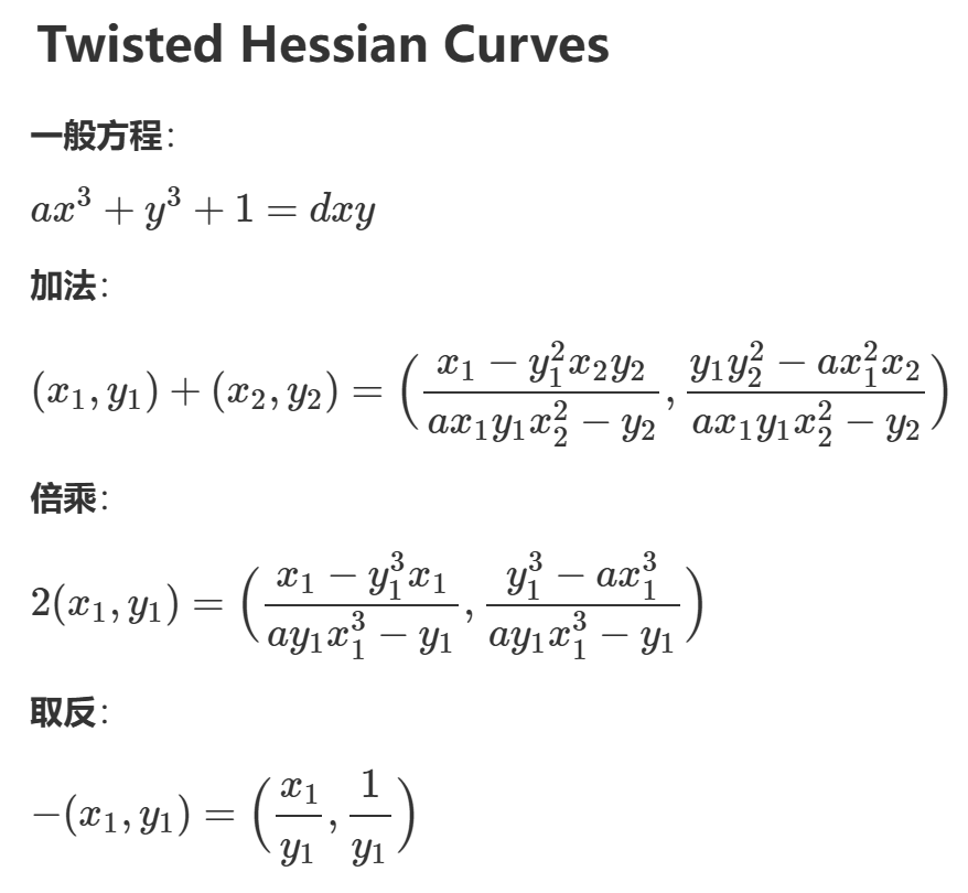
Twisted Hessian曲线(求a)
题目:
from Crypto.Util.number import *
from Crypto.Cipher import AES
from Crypto.Util.Padding import pad
from random import randint
import hashlib
from secrets import flag

def add_THCurve(P, Q):
    if P == (0, 0):
        return Q
    if Q == (0, 0):
        return P
    x1, y1 = P
    x2, y2 = Q
    x3 = (x1 - y1 ** 2 * x2 * y2) * pow(a * x1 * y1 * x2 ** 2 - y2, -1, p) % p
    y3 = (y1 * y2 ** 2 - a * x1 ** 2 * x2) * pow(a * x1 * y1 * x2 ** 2 - y2, -1, p) % p
    return x3, y3

def mul_THCurve(n, P):
    R = (0, 0)
    while n > 0:
        if n % 2 == 1:
            R = add_THCurve(R, P)
        P = add_THCurve(P, P)
        n = n // 2
    return R

p = getPrime(96)
a = randint(1, p)
G = (randint(1,p), randint(1,p))
d = (a*G[0]^3+G[1]^3+1)%p*inverse(G[0]*G[1],p)%p
x = randint(1, p)
Q = mul_THCurve(x, G)
print(f"p = {p}")
print(f"G = {G}")
print(f"Q = {Q}")

key = hashlib.sha256(str(x).encode()).digest()
cipher = AES.new(key, AES.MODE_ECB)
flag = pad(flag,16)
ciphertext = cipher.encrypt(flag)
print(f"ciphertext={ciphertext}")

"""
p = 55099055368053948610276786301
G = (19663446762962927633037926740, 35074412430915656071777015320)
Q = (26805137673536635825884330180, 26376833112609309475951186883)
ciphertext=b"k\xe8\xbe\x94\x9e\xfc\xe2\x9e\x97\xe5\xf3\x04'\x8f\xb2\x01T\x06\x88\x04\xeb3Jl\xdd Pk$\x00:\xf5"
"""
解题思路:
分析Twisted Hessian曲线结构求参数a
- 题目给出了TH曲线的点加法和标量乘法定义以及关键参数
<font style="color:rgb(6, 6, 7);">p,G,Q</font>点,目的是求出<font style="color:rgb(6, 6, 7);">x</font>解这个AES - 但是我们不知道
<font style="color:rgb(6, 6, 7);">a</font>就要想办法求出<font style="color:rgb(6, 6, 7);">a</font>,这里我们可以用Gröbner basis或多元多项式方程组来尝试求a - 分析一下Twisted Hessian曲线结构以此构造多项式
-
已知点
<font style="color:rgb(6, 6, 7);">G=(Gx,Gy)</font>和<font style="color:rgb(6, 6, 7);">Q=(Qx,Qy)</font>,且<font style="color:rgb(6, 6, 7);">Q=x⋅G</font>,可以通过以下步骤求解<font style="color:rgb(6, 6, 7);">a</font>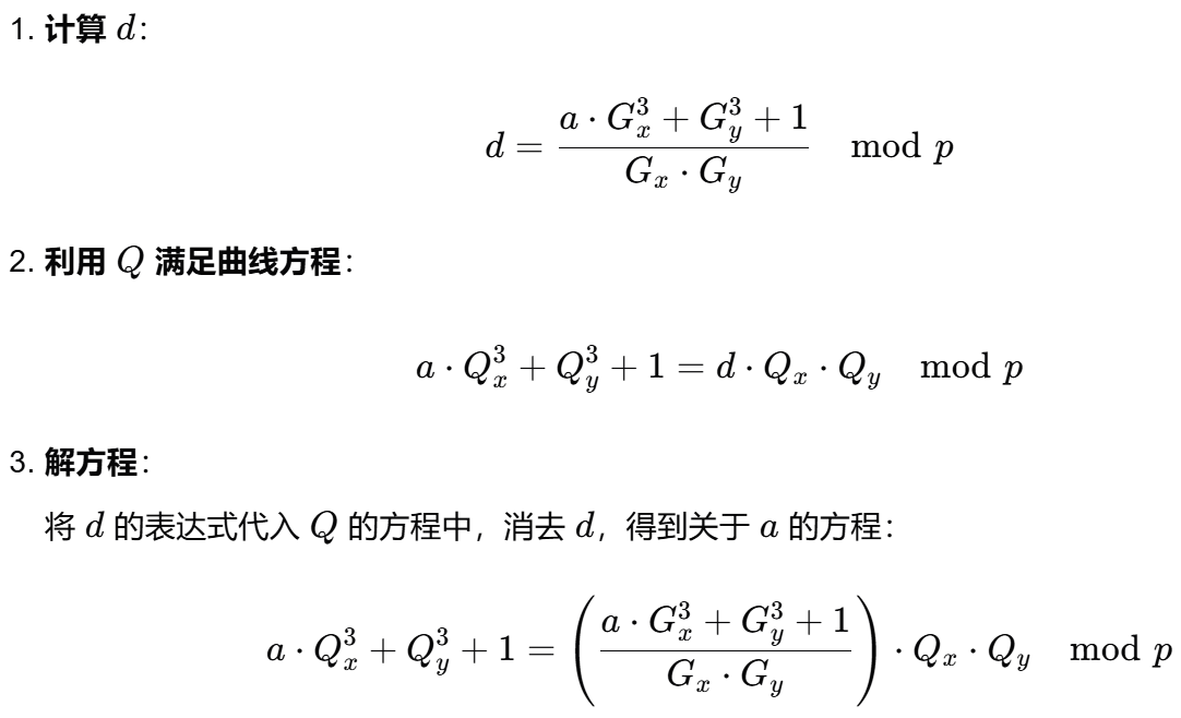
这是一个关于<font style="color:rgb(6, 6, 7);">a</font>的线性方程,可以通过代数方法求解
代码实现:
p = 55099055368053948610276786301
G = (19663446762962927633037926740, 35074412430915656071777015320)
Q = (26805137673536635825884330180, 26376833112609309475951186883)
# 计算 a
Gx, Gy = G
Qx, Qy = Q
GxGy = (Gx * Gy) % p
QxQy = (Qx * Qy) % p
K = (QxQy * pow(GxGy, -1, p)) % p
C2 = (pow(Gy, 3, p) + 1) % p
C1 = (pow(Qy, 3, p) + 1) % p
numerator = (C2 * K - C1) % p
denominator = (pow(Qx, 3, p) - pow(Gx, 3, p) * K) % p
a = (numerator * pow(denominator, -1, p)) % p
print(f'a =', a)
# 计算 d
d = (a * pow(Gx, 3, p) + pow(Gy, 3, p) + 1) * pow(GxGy, -1, p) % p
print(f'd =', d)
'''
a = 39081810733380615260725035189
d = 8569490478014112404683314361
'''
或者直接Gröbner求参数(本质上还是多项式方程组)
代码实现:
p = 55099055368053948610276786301
G = (19663446762962927633037926740, 35074412430915656071777015320)
Q = (26805137673536635825884330180, 26376833112609309475951186883)
# 定义变量
R.<a, d> = PolynomialRing(GF(p))
# 计算 G 和 Q 的相关值
G0, G1 = G
Q0, Q1 = Q
# 构建方程组
eq1 = a * G0^3 + G1^3 + 1 - d * G0 * G1
eq2 = a * Q0^3 + Q1^3 + 1 - d * Q0 * Q1
# 计算 Gröbner 基
I = R.ideal([eq1, eq2])
G = I.groebner_basis()
# 输出 Gröbner 基
print("Gröbner Basis:", G)
# 求解方程组
solutions = I.variety()
print("Solutions:", solutions)
'''
Gröbner Basis: [a + 16017244634673333349551751112, d + 46529564890039836205593471940]
Solutions: [{a: 39081810733380615260725035189, d: 8569490478014112404683314361}]
'''
曲线映射+DLP求解分析
a,d知道了,然后就可以曲线映射后构建出椭圆曲线并使用Pohlig-Hellman算法解决DLP(离散对数)问题求解出<font style="color:rgb(6, 6, 7);">Q=x⋅G</font>中的这个<font style="color:rgb(6, 6, 7);">x</font>- 把
Twisted Herssian上的点映射到Weierstrass上,再求解即可
法1?:首先检查曲线是否奇异,然后将点映射到乘法群并计算离散对数
p = 55099055368053948610276786301
G = (19663446762962927633037926740, 35074412430915656071777015320)
Q = (26805137673536635825884330180, 26376833112609309475951186883)
Gx, Gy = G
Qx, Qy = Q
a = 39081810733380615260725035189
d = 8569490478014112404683314361
##################################################################
# 检查奇异点
rhs = (pow(d, 3, p) * pow(27 * pow(a, 2, p), -1, p)) % p
# 寻找x0的立方根,这里假设存在解
x0 = pow(rhs, (2 * p - 1) // 3, p)
y0 = (3 * a * pow(x0, 2, p) * pow(d, -1, p)) % p
# 映射到乘法群并计算离散对数
t_G = (Gx - x0) * pow(Gy - y0, -1, p) % p
t_Q = (Qx - x0) * pow(Qy - y0, -1, p) % p
x = discrete_log(t_Q, t_G, p)  # 使用离散对数算法求解
print(x)
法2:更方便的是直接通过转为三次齐次方程的方式,再用sage自带的EllipticCurve_from_cubic来做映射
a = 39081810733380615260725035189
p = 55099055368053948610276786301
G = (19663446762962927633037926740, 35074412430915656071777015320)
Q = (26805137673536635825884330180, 26376833112609309475951186883)
########################################################### part1 get d
d = (a*G[0]^3 + G[1]^3 + 1) * inverse_mod(G[0]*G[1], p) % p
########################################################### part2 dlp
R.<x,y,z> = Zmod(p)[]
cubic = a*x^3 + y^3 + z^3 - d*x*y*z
E = EllipticCurve_from_cubic(cubic,morphism=True)
G = E(G)
Q = E(Q)
r = 60869967041981
m = (r*Q).discrete_log(r*G)
print(m)
#14119952000444809975678010351
这个方法和上面那个其实没什么区别,无非上面是sage自动映射的,下面这个是手动映射的
import gmpy2
p = 55099055368053948610276786301
a = 39081810733380615260725035189
G = (19663446762962927633037926740,35074412430915656071777015320)
d = (a*G[0]^3+G[1]^3+1)*gmpy2.invert(G[1]*G[0], p)%p
Q = (26805137673536635825884330180,26376833112609309475951186883)

def calculate_coefficients(a, d):
    d_3 = d*gmpy2.invert(3, p)%p             # d / 3
    tmp = a - d_3**3                    # a - d^3/27
    a0 = 1
    a1 = (-3 * d_3 * gmpy2.invert(tmp, p))%p
    a3 = (-9 * gmpy2.invert(tmp**2, p)) % p
    a2 = (-9 * d_3**2 * gmpy2.invert(tmp**2, p))%p
    a4 = (-27 * d_3 * gmpy2.invert(tmp**3, p))%p
    a6 = (-27 * gmpy2.invert(tmp**4, p))%p
    return [a1, a2, a3, a4, a6]

aa = calculate_coefficients(a, d)
E = EllipticCurve(GF(p), aa)
def Herssian_to_Weierstrass(Point):
    x, y = Point
    u = ((-3 * gmpy2.invert((a - d^3*gmpy2.invert(27, p)), p)*x * gmpy2.invert(d*x*gmpy2.invert(3,p) - (-y) + 1, p))) % p
    v = ((-9 * gmpy2.invert((a - d^3*gmpy2.invert(27, p))^2, p) ) * (-y) * gmpy2.invert(d*x*gmpy2.invert(3,p) - (-y) + 1, p))%p
    return (u, v)

G = E(Herssian_to_Weierstrass(G))
Q = E(Herssian_to_Weierstrass(Q))
x = Q.discrete_log(G)
print(x)
#14119952000444809975678010351
- 但是这时候就出现问题了,为什么得到的
<font style="color:#DF2A3F;">x</font>解不出那个密文 - 找了很多脚本发现
可能是~~discrete_log~~和~~log~~解离散对数的问题
为什么discrete_log和log的结果不同?
-
**discrete_log**函数:这是一个通用的离散对数求解器,适用于多种数学结构;它可能会返回满足条件的任意解,而不一定是最小的解 -
**log**方法:这是椭圆曲线点对象的内置方法,通常会返回最小的标量倍数,因为它针对椭圆曲线的结构进行了优化 -
但是我怎么不能用~~**log**~~(AttributeError: 'EllipticCurvePoint_finite_field' object has no attribute 'log') -
那就用
**discrete_log**吧…… -
欸!?
**x = Q.discrete_log(G)**和**x = discrete_log(Q, G, operation='+')** -
似乎真正的问题在这里
分析<font style="color:rgb(6, 6, 7);">discrete_log</font>函数和椭圆曲线点对象的<font style="color:rgb(6, 6, 7);">discrete_log</font>方法之间的区别
discrete_log函数:
**discrete_log**是一个通用的离散对数求解器,可以用于多种数学结构,包括有限域,椭圆曲线等;它的语法如下:x = discrete_log(Q, G, operation='+')
- 参数:
Q:目标点或目标群元素G:基点或生成元operation:指定群操作的类型,对于椭圆曲线上的点,操作通常是加法('+');对于有限域中的元素,操作通常是乘法('*')
- 适用范围:
- 适用于多种数学结构,包括椭圆曲线和有限域
- 需要显式指定操作类型(加法或乘法)
椭圆曲线点对象的discrete_log方法:
**discrete_log**方法是专门为椭圆曲线上的点设计的离散对数求解器;它的语法如下:x=Q.discrete_log(G)
- 参数:
Q:目标点G:基点或生成元
- 适用范围:
- 仅适用于椭圆曲线上的点
- 不需要显式指定操作类型,因为椭圆曲线上的操作默认是加法
再次进行曲线映射和DLP求解
- 如果这里的两个阶倍数相差太大算起来会非常慢,那么就可以用Pohlig_Hellman算(参考ECC圆锥曲线-Twisted Hessian曲线-2024年"羊城杯"粤港澳大湾区网络安全大赛-TH_Curve)
- 不过这里不适用Pohlig_Hellman求解x不知道为什么
- 只好使用
x = discrete_log(Q, G, operation='+') 具体原理不是太懂
from sage.all import *

# 定义参数
a = 39081810733380615260725035189
p = 55099055368053948610276786301
G = (19663446762962927633037926740, 35074412430915656071777015320)
Q = (26805137673536635825884330180, 26376833112609309475951186883)

# 计算 d
G0, G1 = G
d = (a * G0^3 + G1^3 + 1) * inverse_mod(G0 * G1, p) % p

# 定义椭圆曲线
R = Zmod(p)['x, y, z']; (x, y, z) = R._first_ngens(3)
cubic = a * x^3 + y^3 + z^3 - d * x * y * z
E = EllipticCurve_from_cubic(cubic, morphism=True)

# 将点 G 和 Q 映射到椭圆曲线上
G = E(G)
Q = E(Q)

# 检查点的阶
order_G = G.order()
order_Q = Q.order()
#18366351789351220439989164171
#18366351789351220439989164171

# 验证 Q 的阶是否能整除 G 的阶
if order_Q.divides(order_G):
    print("Q 的阶能整除 G 的阶,离散对数问题可能有解。")
    x = discrete_log(Q, G, operation='+')
    print("离散对数结果:", x)
else:
    print("Q 的阶不能整除 G 的阶,离散对数问题无解。")
'''
Q 的阶能整除 G 的阶,离散对数问题可能有解。
离散对数结果: 2633177798829352921583206736
'''
- 这次得到的结果就是对的,
x的值为2633177798829352921583206736 - 最后AES求解……
解答:
from Crypto.Cipher import AES
import hashlib
from Crypto.Util.Padding import unpad

x = 2633177798829352921583206736
ciphertext=b"k\xe8\xbe\x94\x9e\xfc\xe2\x9e\x97\xe5\xf3\x04'\x8f\xb2\x01T\x06\x88\x04\xeb3Jl\xdd Pk$\x00:\xf5"
key = hashlib.sha256(str(x).encode()).digest()
Cipher = AES.new(key, AES.MODE_ECB)
padded_message = Cipher.decrypt(ciphertext)
message = unpad(padded_message, AES.block_size)
print(message)
#hgame{N0th1ng_bu7_up_Up_UP!}

 浙公网安备 33010602011771号