Advanced Computer Graphics

Lec 1 - Intro

Topics: geometry, rendering, simulation / animation, graphics + AI.

Geometry

3D scanning, curves & surfaces, shapes representations, surface reconstruction, geometry processing (convex decomposition, mesh simplification, surface subdivision, surface editing), surface parameterization & texture mapping.

Rendering

Image formation, cameras, light types, textures & shading, rasterization, ray tracing, non-photorealistic rendering.

Rasterization: Projecting geometry primitives (3D triangles / polygons) onto the screen, breaking projected primitives into fragments (pixels).

Simulation / Animation

Performance capture, character animation, motion retargeting, keyframing, physically based animation.

Graphics + AI

Graphics + (ML / CV / Robotics / NLP / ...).

Lec 2 - Geometry

Basic Geometry Entities

Spline: A type of smooth curve in 2D / 3D completely determined by a set of control points, where a smooth and piecewise polynomial function is fitted to the control points. The curve does not necessarily pass through the control points.

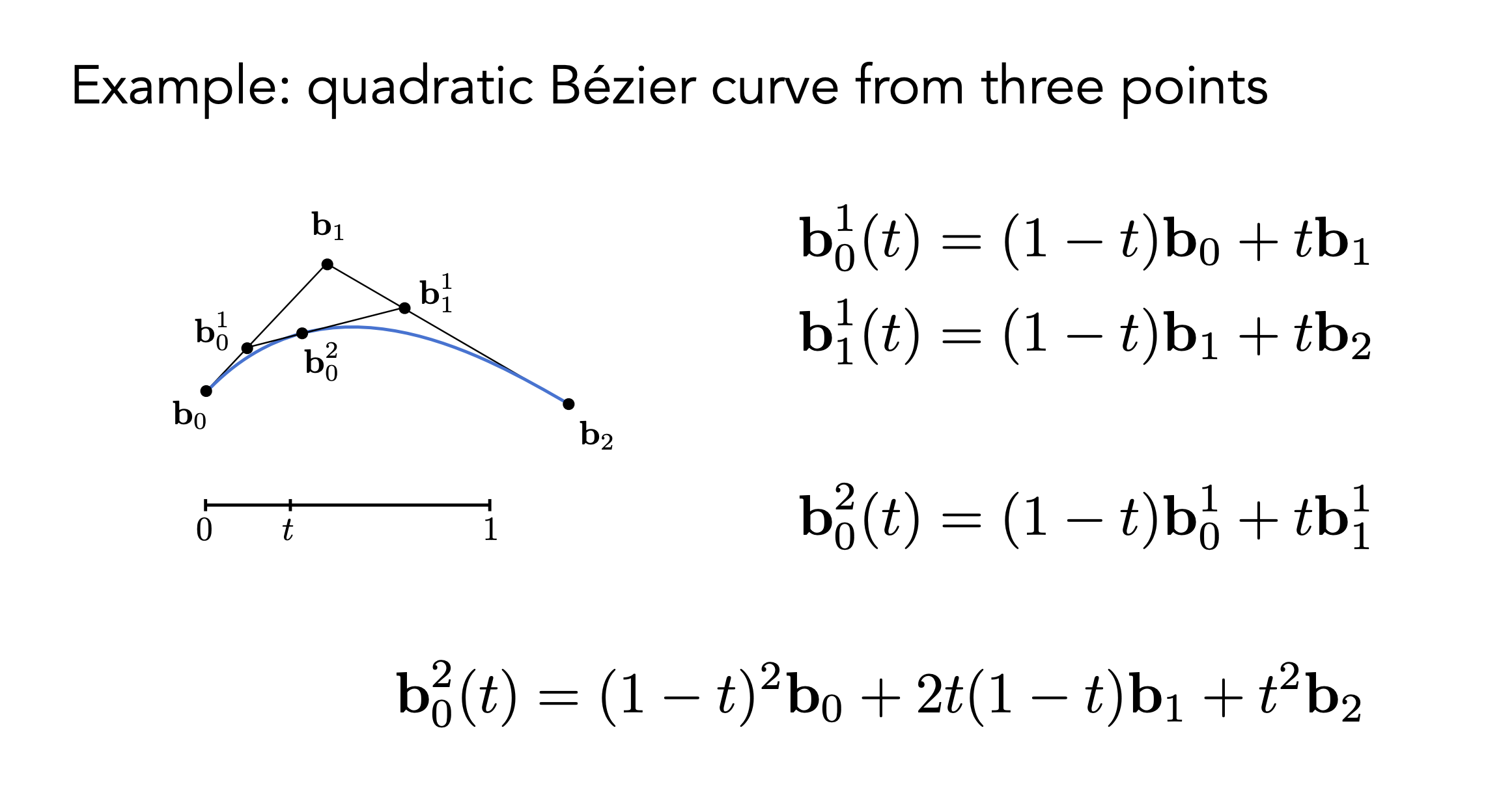
Bézier curve: Given \(n+1\) control points \(P_0, P_1, \ldots, P_n\), we can define the order-\(n\) Bézier curve as $$B_n(t) = \sum_{i=0}^{n} P_i \cdot b_{i,n}(t)$$ where \(b_{i,n}(t)\) are the Bernstein basis polynomials defined as $$b_{i,n}(t) = \binom{n}{i} (1-t)^{n-i} t^i$$ for \(t \in [0,1]\).

Idea: Linear interpolation between control points.

Piecewise Bézier curve: A sequence of Bézier curves joined together. To ensure \(C^0\) continuity (the curve is continuous), the end point of one segment must be the start point of the next segment. To ensure \(C^1\) continuity (the first derivative is continuous), the control points must be aligned.

General spline formulation: \(Q(t) = \mathbf{GBT}(t)\). \(\mathbf G\) is the geometry matrix (control points), \(\mathbf B\) is the spline basis matrix, and \(\mathbf T(t)\) is the power basis vector \((1, t, \cdots, t^n)^{\top}\). Different types of splines have different basis matrices.

Bézier surfaces: $$S(u,v) = \sum_{i=0}^{m} \sum_{j=0}^{n} P_{i,j} \cdot b_{i,m}(u) \cdot b_{j,n}(v).$$

Explicit Geometry Representations

Taxonomy: Rasterized form (regular grids) / geometric from (irregular meshes).

Point cloud: A set of points in 3D space, usually obtained from 3D scanning. Pros: Simple, easy to acquire. Cons: No connectivity information, hard to represent surfaces. Points with orientation are called surfels (shading needs normals).

Polygonal mesh: A collection of vertices, edges, and faces. Piece-wise linear surface representation.

Manifold mesh: 1. Each edge is incident to one or two faces. 2. Faces incident to a vertex form a closed or open fan.

Good triangulation is important (manifold, equi-length)

While real-data 3D are often point clouds, meshes are quite often used to visualize 3D and generate ground truth for machine learning algorithms.

Mesh reconstruction: point cloud \(\to\) mesh.

Watertight manifold surface generation: A surface that completely encloses a volume without any holes or gaps.

Mesh subdivision: Generating a smooth surface from a coarse mesh by iteratively refining the mesh. Each iteration splits each polygonal face into smaller faces and adjusts the vertex positions to approximate a smooth surface.

Mesh simplification: Reducing the number of polygons in a mesh while preserving its overall shape and appearance. Techniques include vertex clustering, edge collapse, and quadric error metrics.

Mesh deformation: Modifying the shape of a mesh by moving its vertices.

Implicit Geometry Representations

Based on classifying points. Easier to test inside / outside.

Distance functions: A function that gives the shortest distance from a point to the surface. The sign of the distance indicates whether the point is inside (negative), outside (positive), or on (zero) the surface.

Lec 3 - Transformation

3D Transformations

To build complex scenes, we need to represent the relative position and orientation of different objects using 3D transformations.

Transformations and Homogeneous Coordinates

Linear transformation: A transformation \(f\) satisfies additivity \(f(\mathbf{x} + \mathbf{y}) = f(\mathbf{x}) + f(\mathbf{y})\) and homogeneity \(f(a\mathbf{x}) = a f(\mathbf{x})\). Linear transformations can be represented by matrix multiplication and composed efficiently. Key property: linear maps take lines to lines.

Basic linear transformations (2D):

• Scale: Uniform scale \(S_a(\mathbf{x}) = a\mathbf{x}\); Non-uniform scale \(S_{\mathbf{s}} = \begin{bmatrix} s_x & 0 \\ 0 & s_y \end{bmatrix}\)
• Rotation: \(R_\theta = \begin{bmatrix} \cos\theta & -\sin\theta \\ \sin\theta & \cos\theta \end{bmatrix}\) (counter-clockwise, preserves vector length)
• Reflection: About y-axis \(Re_y = \begin{bmatrix} -1 & 0 \\ 0 & 1 \end{bmatrix}\); about x-axis \(Re_x = \begin{bmatrix} 1 & 0 \\ 0 & -1 \end{bmatrix}\)
• Shear: In x-direction \(H_{xs} = \begin{bmatrix} 1 & s \\ 0 & 1 \end{bmatrix}\)

Translation: \(T_{\mathbf{b}}(\mathbf{x}) = \mathbf{x} + \mathbf{b}\). Not a linear transformation because it doesn't map origin to origin and violates additivity.

Transformation types:

• Linear: Scale, rotation, reflection, shear (matrix multiplication)
• Affine: Composition of linear transformation and translation (\(f(\mathbf{x}) = A\mathbf{x} + \mathbf{b}\))
• Euclidean (Isometries): Preserve distances (\(|f(\mathbf{x}) - f(\mathbf{y})| = |\mathbf{x} - \mathbf{y}|\)). Includes translation, rotation, reflection
• Rigid body: Distance-preserving transformation that preserves orientation. Includes translation and rotation, excludes reflection

Composition of transformations: Order matters. Scaling then translating yields different result than translating then scaling.

Homogeneous coordinates: Represent a 2D point \((x, y)\) with a 3-vector by adding a third coordinate \(w\). Point: \((x, y) \rightarrow \begin{bmatrix} x \\ y \\ 1 \end{bmatrix}\). Vector: \((x, y) \rightarrow \begin{bmatrix} x \\ y \\ 0 \end{bmatrix}\). All affine transformations can be represented by a single 3x3 matrix multiplication.

Conversion back: Divide by \(w\) coordinate: \(\begin{bmatrix} x \\ y \\ w \end{bmatrix} \rightarrow \begin{pmatrix} x/w \\ y/w \end{pmatrix}\).

Transformation matrices in 2D homogeneous coordinates:

• Scale: \(S = \begin{bmatrix} s_x & 0 & 0 \\ 0 & s_y & 0 \\ 0 & 0 & 1 \end{bmatrix}\)
• Rotation: \(R = \begin{bmatrix} \cos\theta & -\sin\theta & 0 \\ \sin\theta & \cos\theta & 0 \\ 0 & 0 & 1 \end{bmatrix}\)
• Translation: \(T = \begin{bmatrix} 1 & 0 & t_x \\ 0 & 1 & t_y \\ 0 & 0 & 1 \end{bmatrix}\)

Geometric intuition: A 2D affine transformation becomes a 3D linear transformation in homogeneous space. 2D translation is equivalent to a shear transformation in 3D homogeneous coordinate space.

3D transformations: Use 4D homogeneous coordinates. A 3D point \((x, y, z)\) becomes \(\begin{bmatrix} x & y & z & 1 \end{bmatrix}^T\). Translation matrix: $$T_{\mathbf{b}} = \begin{bmatrix} 1 & 0 & 0 & b_x \ 0 & 1 & 0 & b_y \ 0 & 0 & 1 & b_z \ 0 & 0 & 0 & 1 \end{bmatrix}$$

Rotation and \(SO(n)\)

Rotation represents relative orientation between coordinate frames (space frame vs body frame).

Degrees of freedom: Rotation in \(\mathbb{R}^2\) has 1 DoF (angle). Rotation in \(\mathbb{R}^3\) has 3 DoF.

Special Orthogonal Group SO(n): The set of all possible rotations in n-dimensional space. $$SO(n) = {R \in \mathbb{R}^{n \times n} : RR^T = I, \det(R) = 1}$$

Properties:

• Group: Closed under matrix multiplication, has identity element, every element has inverse
• Orthogonal: \(RR^T = I\) means matrix columns are orthonormal vectors. Preserves lengths and angles. Inverse is transpose (\(R^{-1}=R^T\))
• Special: \(\det(R) = 1\) ensures pure rotation, not reflection (which has \(\det = -1\))

Topology of rotation space: SO(2) has topology of a circle. SO(3) has more complex topology. These spaces are not topologically equivalent to Euclidean space \(\mathbb{R}^n\). Implication: No perfect bijection exists between simple network output (e.g., vector in \(\mathbb{R}^3\)) and rotation in SO(3). This can cause neural networks to make poor predictions (e.g., angles 0 and \(2\pi\) are close but have distant parameter outputs). Requires careful design of rotation representations for machine learning.

3D Rotation Representations

Euler angles: Any 3D rotation described as sequence of three rotations about principal axes (e.g., X, then Y, then Z). Matrix form: \(R = R_z(\gamma)R_y(\beta)R_x(\alpha)\). Intuitive (roll, pitch, yaw). Drawback: Gimbal lock. When middle rotation angle is \(\pm 90^\circ\), first and third rotation axes align, losing one degree of freedom. Representation is not unique for certain rotations.

Axis-angle: Euler's rotation theorem states any rotation in SO(3) is equivalent to single rotation by angle \(\theta\) about fixed axis \(\hat{\omega}\). Gives 3-parameter representation (2 for axis direction, 1 for angle), often encoded as rotation vector \(\vec{\omega} = \theta \hat{\omega}\).

Conversion to rotation matrix (Rodrigues' formula): $$R(\hat{\omega}, \theta) = I + (\sin\theta)[\hat{\omega}] + (1-\cos\theta)[\hat{\omega}]^2$$ where \([\hat{\omega}]\) is skew-symmetric matrix corresponding to cross-product with \(\hat{\omega}\). Can also be written as matrix exponential \(R = e^{[\vec{\omega}]} = e^{\theta[\hat{\omega}]}\).

Conversion from rotation matrix: $$\theta = \arccos\left(\frac{\text{tr}(R)-1}{2}\right), \quad [\hat{\omega}] = \frac{R - R^T}{2\sin\theta}$$

Not unique: \(\text{Rot}(\hat{\omega}, \theta) = \text{Rot}(-\hat{\omega}, -\theta)\), but can be made unique by restricting \(\theta \in [0, \pi]\).

Quaternions: 4-dimensional extension of complex numbers. Definition: \(q = w + x\mathbf{i} + y\mathbf{j} + z\mathbf{k}\), where \(\mathbf{i}^2 = \mathbf{j}^2 = \mathbf{k}^2 = \mathbf{ijk} = -1\). Unit quaternion (where \(\|q\| = w^2+x^2+y^2+z^2 = 1\)) represents 3D rotation. 4-parameter representation with one constraint, giving 3 DoF.

Conversion from axis-angle: Rotation by \(\theta\) around axis \(\hat{\omega}=(w_x, w_y, w_z)\) is $$q = \left(\cos(\theta/2), \sin(\theta/2)w_x, \sin(\theta/2)w_y, \sin(\theta/2)w_z\right)$$

Properties: Composition is quaternion multiplication. Compact and computationally efficient. Avoids gimbal lock. Good numerical stability (popular for interpolation/slerp). Drawback: Less intuitive. Double-covering property: \(q\) and \(-q\) represent same rotation.

Summary:

• Rotation matrix: 9 params, redundant, can drift. Inverse is transpose, composition is multiplication
• Euler angles: Intuitive, suffers from gimbal lock. Complicated inverse and composition
• Axis-angle: Intuitive, complicated composition. Inverse is negate angle/axis
• Quaternion: Standard in practice. Compact, efficient, no gimbal lock. Inverse is conjugate, composition is multiplication

Viewing Transformation

Graphics pipeline: Modeling transformation (object space → world space) → View/camera transformation (world space → camera space) → Projection transformation (3D → 2D) → Viewport transformation (NDC → screen coordinates).

View/camera transformation: Transform world so camera is at canonical origin (at origin, looking down -Z axis, Y up). Camera definition: Position \(\vec{e}\), look-at direction \(\hat{g}\), up vector \(\hat{t}\).

View matrix \(M_{view}\): Transforms vertices from world space to camera space. Composed of translation and rotation:

1. Translate world by \(-\vec{e}\) to move camera to origin (\(T_{view}\))
2. Rotate world so camera axes \((\hat{g}\times\hat{t}, \hat{t}, -\hat{g})\) align with world (X, Y, Z) axes (\(R_{view}\))
3. \(M_{view} = R_{view} \cdot T_{view}\)

Combined Model-View matrix is often called ModelView matrix in OpenGL.

Projection transformation: Maps 3D camera-space view volume into 2D canonical view volume (NDC cube from -1 to 1). Orthographic projection: Preserves parallel lines and relative sizes. Perspective projection: Models realistic viewing. Objects farther away appear smaller. Non-affine transformation achieved using homogeneous \(w\) coordinate.

Viewport transformation: Maps NDC cube to screen coordinates. Affine transformation that scales and translates \([-1, 1]\) coordinates to pixel range \([x, x+\text{width}]\) and \([y, y+\text{height}]\).

Lec 4 - Learning + Geometry

Perspective Projection

Perspective projection mimics human vision where objects farther away appear smaller. Achieved in two steps: 1. Transform viewing frustum (truncated pyramid) into canonical cuboid (often \([-1, 1]^3\)). 2. Perform orthographic projection on this cuboid.

Deriving perspective matrix: Using similar triangles, projected coordinates on near plane at distance \(n\) are: $$y' = \frac{n}{z} y, \quad x' = \frac{n}{z} x$$

In homogeneous coordinates, transformation becomes: $$\begin{pmatrix} x \ y \ z \ 1 \end{pmatrix} \xrightarrow{M_{persp}} \begin{pmatrix} nx \ ny \ \text{unknown} \ z \end{pmatrix}$$

After homogeneous divide (dividing by \(z\)), we get correct \(x' = nx/z\) and \(y' = ny/z\).

Finding third row: Any point on near plane (\(z=n\)) maps to \(n\), any point on far plane (\(z=f\)) maps to \(f\). Let third row be \([0 \quad 0 \quad A \quad B]\). System of equations:

• Near plane: \(An + B = n^2\)
• Far plane: \(Af + B = f^2\)

Solution: \(A = n + f\) and \(B = -nf\).

Frustum "squish" matrix:

\[M_{persp \rightarrow ortho} = \begin{bmatrix} n & 0 & 0 & 0 \\ 0 & n & 0 & 0 \\ 0 & 0 & n+f & -nf \\ 0 & 0 & 1 & 0 \end{bmatrix} \]

Orthographic projection matrix (maps cuboid to NDC cube \([-1, 1]^3\)):

\[M_{ortho} = \begin{bmatrix} \frac{2}{r-l} & 0 & 0 & -\frac{r+l}{r-l} \\ 0 & \frac{2}{t-b} & 0 & -\frac{t+b}{t-b} \\ 0 & 0 & \frac{2}{n-f} & -\frac{n+f}{n-f} \\ 0 & 0 & 0 & 1 \end{bmatrix} \]

Final perspective projection matrix: \(M_{persp} = M_{ortho} \cdot M_{persp \rightarrow ortho}\).

Z-fighting: Perspective transformation non-linearly maps z-values, compressing far values into smaller range. Causes loss of depth buffer precision. Surfaces very close together incorrectly appear to intersect or flicker.

AI and 3D Graphics

Success in 2D deep learning fueled by mature 2D datasets (ImageNet, MSCOCO) and successful backbones (AlexNet, VGG, ResNet, Vision Transformers).

Rise of AI + 3D: Key research areas include large-scale 3D datasets, deep 3D understanding, and deep 3D synthesis. Trending topics at major conferences: "3D from multi-view" and "3D from single images".

Geometric Datasets

Object-centric datasets:

• Early datasets (pre-2014): Princeton Shape Benchmark with few thousand models
• ShapeNet (2015): Over 3 million models across 4,000+ object classes (~100× larger than previous datasets). Rich in attributes: semantic categories linked to WordNet, pose, part hierarchies, material, size, affordances
• PartNet: Fine-grained, instance-level, hierarchical part annotations
• Other datasets: Thingi10K (3D printing), ABC (CAD models), Objaverse-XL (over 10 million objects)

Scene-level datasets:

• Indoor scenes: ScanNet (real scanned indoor scenes with RGBD data, camera poses, semantic segmentations), ScanNet++ (high-fidelity with sub-millimeter geometry and DSLR imagery), SceneNet (synthetic photorealistic indoor scenes)
• 4D datasets (3D + Time): Autonomous driving (Waymo Open Dataset, Semantic Kitti), human-object interaction (HOI4D, BEHAVE, EgoBody)

Virtual environments: SAPIEN and ThreeDWorld provide simulated environments for training and testing agents.

Data-Driven Shape Analysis

Shape analysis: Learning to predict label or condition \(c\) given shape \(S\), modeling \(P(c|S)\). Includes classification and segmentation. Challenge: designing neural networks for various 3D representations.

Multi-view CNNs (MVCNN): Render 3D object from multiple viewpoints, apply 2D CNN to each image, aggregate features (view pooling) for global shape descriptor. Pros: Leverage powerful pre-trained 2D networks, strong performance. Cons: Requires rendering, struggles with noisy/incomplete point clouds.

Volumetric (3D CNNs): Represent shape as occupancy grid of voxels, apply 3D convolutions. Cons: Computational and memory cost grows cubically with resolution (\(O(L^3)\)), prohibitive. Forces low resolutions (32³ or 64³), significant information loss.

Sparse volumetric methods: Most 3D space is empty. Only store and compute on occupied voxels near surface. Sparse convolution (MinkowskiEngine, SparseConvNet) only computes outputs for non-zero input locations. Octrees (O-CNN): Hierarchical data structure recursively partitioning space into eight children, efficiently representing sparse data.

Point-based methods (PointNet): Challenge: Point clouds are unordered sets, network must be invariant to permutations. Architecture: 1. Process each point independently with shared MLP to high-dimensional feature space. 2. Symmetric aggregation (max pooling) across points for global feature vector. 3. MLP processes global vector for tasks like classification. Limitations: Does not capture local geometric structures. PointNet++: Improves by recursively applying PointNet to local neighborhoods, learning hierarchical features at multiple scales.

Graph-based methods: Treat point cloud as graph (points are nodes, connections to neighbors are edges), apply Graph Neural Networks (GNNs). Challenge: Standard message-passing GNNs not invariant to sampling density.

Spectral CNNs: Apply convolutions in spectral domain of shape's graph Laplacian. Provides invariance to isometric (length-preserving) deformations. Limitation: Fails for non-isometric shapes (spectral domains not aligned).

Data-Driven Shape Synthesis

Shape synthesis: Learning to generate new shapes, often conditioned on input \(c\), modeling \(P(S|c)\).

Single-view 3D modeling: Reconstruct 3D shape of object from single 2D image. Ill-posed problem: Single 2D projection has infinite possible 3D explanations (Ames Room illusion). Solution: Data-driven priors. Real world has strong regularities. Models learn regularities from large datasets to predict most plausible 3D shape.

Evolution of approaches:

• Early work: Model-based fitting with limited templates or geometric primitives matched to image features
• Modern data-driven view: Learn expressive inference system (neural network) over large training dataset (ShapeNet) to directly map image to 3D output

Examples:

• 2D to 2.5D (depth prediction): Predict depth map from single image. Challenging due to scale/depth ambiguity (small close object looks identical to large far object). Modern methods use scale-invariant loss functions
• Image-to-3D object modeling: Supervised learning on pairs of [image, 3D model] to learn direct mapping. Modern systems like Instant3D perform fast text-to-3D generation

Lec 5 - Rasterization

Learning to Predict 3D from 2D

Learning to predict 3D structure from 2D image: Canonical task in 3D computer vision, framed as supervised learning.

Learning recipe:
0. Decide on 3D representation (model) and learning objective (loss function)

1. Collect large dataset of [image, 3D] pairs
2. Train predictor (e.g., CNN) to map images to chosen 3D representation
3. Use predictor for inference

Learning from synthetic data: Synthetic datasets like ShapeNet useful for debugging but have limitations. Realism gap: Simple appearances and materials. Bias: Biased towards rigid, man-made object categories. Progress on synthetic data doesn't always translate to real-world tasks.

Learning different representations:

• Volumetric 3D: Encoder-decoder network predicts voxel grid from image. Training on renderings with random backgrounds helps generalization. Hierarchical methods (Octrees) improve efficiency by only representing occupied space
• Implicit representations (Occupancy Networks): Network learns function determining if arbitrary point \((x, y, z)\) is inside or outside shape
• Point clouds: Naive L2 loss between predicted and ground-truth points is flawed (assumes point-to-point correspondence, doesn't exist for unordered sets). Permutation-invariant objective needed. Chamfer distance: $$d_{CD}(S_1, S_2) = \sum_{x \in S_1} \min_{y \in S_2} |x-y|2^2 + \sum \min_{x \in S_1} |x-y|_2^2$$
• Meshes (via deformation): Start with template mesh (e.g., sphere), network predicts 3D displacement for each vertex, deforming into target shape while keeping connectivity fixed. Training objectives: Data term (Chamfer distance on sampled points) combined with smoothness regularization (e.g., Laplacian loss) to encourage well-formed meshes
• Specialized models (humans with SMPL): For articulated objects like human body, parametric models like SMPL (Skinned Multi-Person Linear Model). Disentangle identity-dependent shape from motion-dependent pose for structured and realistic predictions

Introduction to Rasterization

After viewing transformation pipeline (Model → View → Projection), geometric primitives (usually triangles) are in canonical view volume. Rasterization: Converting continuous geometric primitives into discrete pixel values on screen.

Screen: Discretized 2D canvas. Pixel: Picture element, smallest unit of digital image, assumed square with uniform color. Resolution: Size of pixel array (e.g., 1920×1080). Raster: German for "grid". Rasterize: Draw onto screen.

Display technologies:

• Historical: Cathode Ray Tubes (CRTs) used electron beam to draw image line-by-line (raster scan)
• Modern flat panels: LCD (Liquid Crystal Display) blocks/transmits light from backlight via liquid crystals. OLED, LED: Each pixel is light-emitting diode. E-Ink: Uses charged black and white particles
• Frame buffer: Region of memory storing color value for every pixel on screen

Rasterizing a Triangle

Triangles are fundamental shape primitive: Guaranteed to be planar, have well-defined interior, allow smooth interpolation of values (e.g., color) using barycentric coordinates.

Rasterization problem: Given triangle defined by vertices' 2D screen coordinates, which pixels should be filled to approximate it?

Rasterization as 2D sampling: Define binary function inside(tri, x, y) that is 1 if point \((x, y)\) is inside triangle, 0 otherwise. Evaluate function for center of each pixel. Point is inside triangle if on same side of all three edges. Check using 2D cross product or implicit equation of line defined by each edge.

Optimization: Bounding box. Instead of iterating over all pixels on screen, only test pixels within triangle's axis-aligned bounding box.

Antialiasing

Simple point sampling at pixel centers leads to aliasing or "jaggies" (stark, jagged edges).

Aliasing: Occurs when signal sampled at frequency too low to capture details. High-frequency details incorrectly appear as low-frequency patterns. Spatial aliasing: Jaggies in images. Temporal aliasing: Wagon-wheel effect in videos.

Solution: Pre-filtering. Remove high frequencies from signal before sampling.

Signal processing view:

1. Sharp edge represents very high frequencies
2. Sampling in spatial domain equivalent to replicating signal's spectrum in frequency domain
3. If sampling rate too low, replicated spectra overlap, causing aliasing
4. Pre-filtering applies low-pass filter (blurring) to original continuous signal. Removes high frequencies, narrowing spectrum so replicas don't overlap after sampling

Convolution theorem: Filtering in frequency domain equivalent to convolution in spatial domain. Box filter (averaging over small window) is simple low-pass filter.

Antialiasing in practice: MSAA (Multisample Antialiasing). Pre-filtering means computing average coverage of triangle within each pixel's square area. Exact area calculation is complex. MSAA is practical approximation:

1. Supersample: Take multiple samples (e.g., 2×2 or 4×4) at different locations inside each pixel
2. Test: For each sample, test if inside triangle
3. Average: Final pixel color is average of results. If \(k\) out of \(N\) samples inside red triangle, pixel color becomes \(k/N \times \text{red}\)

Results in pixels along edges having intermediate colors, creating smoother appearance.

Z-Buffering

When multiple triangles overlap in scene, need to determine which is visible at each pixel.

Painter's algorithm: Sort all triangles by depth, draw from back to front, overwriting previously drawn pixels. Problems: Requires sort (\(O(N \log N)\)), slow. Fails for complex cases with intersecting or cyclically overlapping triangles.

Z-buffer algorithm: Standard hardware-accelerated solution in modern GPUs. For each pixel, store depth (z-value) of closest object found so far.

Data structures:

• Frame buffer: Stores color values for each pixel
• Depth buffer (Z-buffer): Additional buffer of same size storing depth value for each pixel

Algorithm:

1. Initialize every value in depth buffer to \(+\infty\)
2. For each triangle \(T\) in scene:
3. For each sample \((x, y)\) that \(T\) covers:
   • Calculate depth \(z\) of triangle at sample point
   • If \(z < \text{zbuffer}[x][y]\):
     • Triangle is closer than what's been seen before
     • Update depth: \(\text{zbuffer}[x][y] = z\)
     • Update color: \(\text{framebuffer}[x][y] = \text{color of } T\)

Complexity: \(O(N)\) for \(N\) triangles (assuming constant screen coverage per triangle). Depth test performed per-pixel, effectively sorting depths in linear time. Result independent of order triangles are processed.

Lec 6 - Shading

Shading Fundamentals

Shading: Process of determining color of point on surface.

Perceptual observations: Different types of lighting and reflection. Specular highlights: Bright mirror-like reflections of light source. Diffuse reflection: Light scatters uniformly in all directions, reveals object's intrinsic color. Ambient lighting: Light from all directions, illuminates areas not directly hit by light source.

Shading is local: Computes light reflected toward camera at specific shading point. Does not account for how other objects block light. Local shading models do not generate shadows. Shading is distinct from shadowing.

Inputs for local shading model:

• Viewer direction \(\mathbf{v}\): Vector from shading point to camera
• Surface normal \(\mathbf{n}\): Vector perpendicular to surface at shading point
• Light direction \(\mathbf{l}\): Vector from shading point to light source (calculated for each light)
• Surface parameters: Color, shininess, etc.

Diffuse Reflection (Lambertian)

Principle: Light scattered uniformly in all directions. Surface color appears same from all viewing directions.

Lambert's cosine law: Light energy received by surface depends on angle of incidence. Energy proportional to cosine of angle \(\theta\) between light direction \(\mathbf{l}\) and surface normal \(\mathbf{n}\). Light per unit area proportional to \(\cos \theta = \mathbf{n} \cdot \mathbf{l}\) (assuming unit vectors). Why regions on Earth receive less solar energy during winter: Sun's rays strike surface at more oblique angle.

Light falloff: Intensity of light from point source decreases with distance. Inverse square law: $$I' = \frac{I}{r^2}$$ where \(I\) is intensity at distance 1.

Lambertian (diffuse) shading model: Independent of view direction. $$L_d = k_d \left( \frac{I}{r^2} \right) \max(0, \mathbf{n} \cdot \mathbf{l})$$

Where:

• \(k_d\) (diffuse coefficient): Intrinsic color of surface
• \((I/r^2)\): Energy arriving at shading point (light intensity with falloff)
• \(\max(0, \mathbf{n} \cdot \mathbf{l})\): Energy received by shading point (Lambert's cosine law). Max ensures light from behind (\(\mathbf{n} \cdot \mathbf{l} < 0\)) doesn't contribute

Specular Term (Blinn-Phong Model)

Principle: Specular reflection is view-dependent. Brightest when viewing direction close to mirror reflection direction.

Blinn-Phong approach: Uses half vector \(\mathbf{h}\) (bisector of viewer direction \(\mathbf{v}\) and light direction \(\mathbf{l}\)) instead of reflection vector. Specular highlights strong when half vector \(\mathbf{h}\) close to surface normal \(\mathbf{n}\). More computationally efficient than original Phong model.

Half vector: $$\mathbf{h} = \frac{\mathbf{v} + \mathbf{l}}{|\mathbf{v} + \mathbf{l}|}$$

Blinn-Phong specular term: $$L_s = k_s \left( \frac{I}{r^2} \right) \max(0, \mathbf{n} \cdot \mathbf{h})^p$$

Where:

• \(k_s\) (specular coefficient): Color/intensity of highlight
• \((I/r^2)\): Energy arriving at point
• \(\max(0, \mathbf{n} \cdot \mathbf{h})^p\): Measures how near half-vector is to normal
• \(p\) (shininess exponent): Controls size of highlight. Higher \(p\) creates smaller, sharper highlight (narrower reflection lobe), simulating shinier surface

Ambient Term

Principle: Approximation for indirect illumination (light bouncing off other surfaces). Adds constant color to prevent shadows from being completely black. "Fake" term, doesn't depend on light position or viewer direction.

\[L_a = k_a I_a \]

Where:

• \(k_a\) (ambient coefficient): Surface's ambient color
• \(I_a\): Intensity of ambient light

Blinn-Phong Reflection Model

Complete model combines ambient, diffuse, and specular terms: $$L = L_a + L_d + L_s = k_a I_a + k_d \left( \frac{I}{r^2} \right) \max(0, \mathbf{n} \cdot \mathbf{l}) + k_s \left( \frac{I}{r^2} \right) \max(0, \mathbf{n} \cdot \mathbf{h})^p$$

Summation performed for every light source in scene.

Shading Frequencies

Smoothness of shaded object depends on how often shading calculation performed.

Flat shading (per-triangle): One normal vector for entire triangle. Shading calculation performed once per triangle. Result is faceted, not good for smooth surfaces.

Gouraud shading (per-vertex): Each vertex has normal vector. Shading calculation performed at each vertex to get vertex colors. Colors interpolated across triangle face. Smoother than flat shading but can miss specular highlights in middle of triangle.

Phong shading (per-pixel): Normal vectors interpolated across triangle face for each pixel. Full shading model computed at every pixel. Produces highest quality, smooth results. Note: Phong shading is different from Blinn-Phong reflectance model.

Defining Normals

Per-vertex normals:

• Geometric primitives (sphere): Derived from underlying geometry
• Triangle meshes: Inferred by averaging face normals of all triangles sharing vertex: $$N_v = \frac{\sum_i N_i}{|\sum_i N_i|}$$

Per-pixel normals (for Phong shading): Vertex normals interpolated across triangle using barycentric interpolation. Crucial to normalize interpolated vector at each pixel before using in shading calculation.

Graphics Pipeline

Graphics pipeline: Sequence of stages transforming 3D scene into 2D image.

1. Application stage: CPU prepares data (vertices, textures) for GPU
2. Vertex processing: Applies Model, View, Projection transformations to position vertices in screen space. Input: Vertices in 3D space. Output: Transformed vertices
3. Triangle processing: Connects vertices to form triangles
4. Rasterization: Determines which pixels covered by each triangle ("sampling triangle coverage"). Input: Triangles in screen space. Output: Fragments (potential pixels)
5. Fragment processing (fragment shader): Shading (computes color using shading models like Blinn-Phong, per-pixel shading happens here), texturing (applies textures), Z-buffer visibility tests. Input: Fragments. Output: Shaded fragments (pixels with color and depth)
6. Framebuffer operations: Final shaded fragments written to framebuffer, blending or replacing existing pixel values
7. Display: Final image in framebuffer sent to screen

Shader programs: Modern GPUs have programmable stages (vertex and fragment processing). Programmed using shader languages like GLSL, HLSL. Fragment shader executes once per fragment, performs texture lookups for material color, then lighting calculations to output final color.

Texturing

Texture mapping: Allows applying image (texture) to surface to define properties (like color) at different points. Instead of constant diffuse coefficient \(k_d\), varies across surface (e.g., wood grain, patterns on ball).

Core idea: Surface lives in 3D world space. Gets projected to 2D screen space. Every point on 3D surface can be mapped to 2D coordinate on image called texture space. Coordinates denoted \((u, v)\).

Texture mapping process:

1. UV parameterization: Assign \((u,v)\) texture coordinates to each vertex of 3D model. "Flattens" or "unwraps" 3D object onto 2D plane. Goal: Minimize distortion
2. Interpolation: During rasterization, \((u,v)\) coordinates interpolated across triangle for each fragment using barycentric coordinates
3. Texture lookup: In fragment shader, interpolated \((u,v)\) coordinate used to look up color value from texture image. Color used in shading calculation (e.g., as diffuse coefficient \(k_d\))

Barycentric Coordinates

Coordinate system for triangles \((\alpha, \beta, \gamma)\) expressing any point \(P(x,y)\) inside triangle (vertices \(A\), \(B\), \(C\)) as weighted average: $$P = \alpha A + \beta B + \gamma C$$

Constraints: $$\alpha + \beta + \gamma = 1, \quad \alpha, \beta, \gamma \ge 0 \text{ if } P \text{ inside triangle}$$

Geometric viewpoint: Coordinates proportional to areas of sub-triangles formed by point \(P\) and triangle's edges: $$\alpha = \frac{\text{Area}(PBC)}{\text{Area}(ABC)}, \quad \beta = \frac{\text{Area}(PAC)}{\text{Area}(ABC)}, \quad \gamma = \frac{\text{Area}(PAB)}{\text{Area}(ABC)}$$

Usage: Any attribute defined at vertices (color, normals, texture coordinates) can be smoothly interpolated across triangle: $$\text{Value}_P = \alpha \cdot \text{Value}_A + \beta \cdot \text{Value}_B + \gamma \cdot \text{Value}_C$$

Important caveat: Barycentric coordinates in 2D screen space not invariant under 3D perspective projection. Perspective-correct interpolation required for accurate results in 3D rendering.

Texture Queries

Texel: Pixel in texture map.

Texture magnification: Single texel stretched over multiple screen pixels. Happens when viewer very close to textured surface.

• Nearest neighbor: Blocky appearance
• Bilinear interpolation: Smooths result by weighted average of 4 nearest texels. Good and common solution
• Bicubic interpolation: Uses 16 nearest texels for smoother, higher-quality result but higher computational cost

Texture minification: Multiple texels compressed into single screen pixel. Happens when textured surface far away.

• Problem: Point sampling leads to severe aliasing artifacts (Moiré patterns, jaggies)
• Correct solution: Average color values of all texels within footprint of single screen pixel. Computationally expensive

Mipmapping

Mip from Latin "multum in parvo" (multitude in small space). Efficient solution for minification.

Technique: Pre-calculate and store sequence of downsampled, pre-filtered versions of texture. Each level half resolution of previous (e.g., 128×128, 64×64, 32×32, ..., 1×1). Mipmap pyramid.

Storage overhead: Additional storage for all mipmap levels only 1/3 of original texture size. Total size \(= N + N/4 + N/16 + \cdots = N \times (4/3)\).

How it works:

1. Compute mipmap level \(D\): For each pixel, estimate size of footprint in texture space. Used to calculate appropriate mipmap level: $$D = \log_2 L$$ where \(L\) is length of pixel footprint
2. Query mipmap:
   • Simple mipmapping: Round \(D\) to nearest integer level, perform bilinear interpolation on that level's texture. Can cause abrupt jump in quality between levels
   • Trilinear interpolation: Perform bilinear interpolation on two closest mipmap levels (\(\lfloor D \rfloor\) and \(\lceil D \rceil\)), then linearly interpolate between those two results based on fractional part of \(D\). Produces smoother result

Limitation: Mipmaps approximate pixel footprint as square. When surface viewed at grazing angle, footprint is long and thin (anisotropic). Square approximation leads to overblur.

Anisotropic filtering: Advanced technique handling non-square (anisotropic) footprints better. Can be visualized as sampling from multiple mipmap levels or using rectangularly filtered textures (ripmaps). Produces sharper results for surfaces at grazing angles but more computationally expensive than trilinear mipmapping.

Applications of Textures

In modern GPUs, texture is general-purpose data structure for memory + fast, filtered range queries.

• Environment mapping: Texture (often cube map) stores lighting from all directions at point in scene. Used to render realistic reflections on objects
• Bump mapping / normal mapping: Texture stores height or normal vector perturbations. Perturbs surface normal during shading to create illusion of fine surface detail without adding more geometry
• Displacement mapping: Height-map texture used to actually move vertices of mesh, creating real geometric detail
• Procedural and 3D textures: Textures generated by mathematical function (procedural) or exist in 3D volumes (e.g., marble, wood, medical volume rendering)

Shadow Mapping

Common rasterization-based technique for adding shadows to scene.

Key idea: Point NOT in shadow if visible from both light source and camera.

Algorithm (two-pass):

Pass 1: Render from light's perspective:

1. Position "camera" at light source
2. Render scene from this perspective
3. Store depth of each fragment in texture. This texture is shadow map. Contains distance from light to nearest surface in every direction

Pass 2: Render from camera's perspective:

1. Render scene normally from main camera's point of view
2. For each fragment being shaded:
   • Calculate position in world space
   • Transform world-space position into light's coordinate system (same system used in Pass 1)
   • Gives coordinate \((u, v)\) and depth \(d_{\text{current}}\) from light's perspective
   • Look up depth \(d_{\text{shadowmap}}\) stored in shadow map at coordinate \((u, v)\)
   • Compare depths:
     • If \(d_{\text{current}} > d_{\text{shadowmap}}\) (plus small bias to avoid self-shadowing artifacts), another object is closer to light. Current fragment is in shadow
     • If \(d_{\text{current}} \approx d_{\text{shadowmap}}\), fragment is visible to light and is lit

Problems:

• Hard shadows: Only produces hard-edged shadows (point lights). Soft shadows (area lights) not directly handled
• Resolution dependent: Quality depends on shadow map resolution. Low resolution leads to blocky or jagged shadow edges ("jaggies")
• Floating point precision: Comparing depth values can lead to precision issues, causing "shadow acne" (surface incorrectly shadows itself). Small bias typically added to mitigate

Beyond rasterization: Ray tracing. Different rendering technique simulating path of light rays. Physically more accurate but computationally very slow. Naturally handles complex phenomena: soft shadows, glossy reflections, indirect illumination.

Lec 7 - Ray Tracing I

Introduction to Ray Tracing

Ray tracing: Rendering technique fundamentally different from rasterization. Excels at simulating global illumination effects difficult with rasterization: soft shadows (shadows with soft edges from area light sources), glossy reflections (blurred, imperfect reflections on semi-smooth surfaces), indirect illumination (light bouncing off surfaces to illuminate other objects).

Ray Casting

Ray casting: Simplest form of ray tracing. Involves shooting rays from camera to determine what is visible.

Generating eye rays: Using pinhole camera model, for each pixel:

1. Eye ray generated, starting from eye point (camera position)
2. Ray directed to pass through center of current pixel on image plane
3. Find all intersections between ray and objects in scene
4. Closest intersection point is visible to camera for that pixel

Shading pixels: Once closest intersection point found, color determined by local shading calculation (e.g., Blinn-Phong). Requires surface normal at intersection point and direction to light source(s).

Adding shadows with shadow rays: Check if path from intersection point to light source is blocked. Cast shadow ray from intersection point towards light source. If shadow ray intersects another object before reaching light, point is in shadow for that light. If shadow ray reaches light source unobstructed, point is illuminated.

Recursive (Whitted-Style) Ray Tracing

Introduced by Turner Whitted (1980). Extends ray casting to handle global effects like perfect reflections and refractions by recursively tracing new rays.

Recursive process:

1. Primary ray: Initial ray cast from eye through pixel
2. Local illumination: When primary ray hits object, color first determined by local shading (diffuse and specular) and shadow checks
3. Secondary rays:
   • If surface reflective (mirror): Generate reflection ray, trace recursively
   • If surface refractive (glass, water): Generate refraction ray, trace recursively
4. Color contribution: Final pixel color is sum of local illumination plus weighted colors returned from recursive calls for reflection and refraction rays

Process repeated for secondary rays, creating tree of rays bouncing around scene. Recursion stops after certain depth to prevent infinite loops.

Depth of recursion = 0: Basic ray casting with only local illumination. Depth = 1: Includes one level of reflection/refraction. Depth > 1: Allows multiple bounces, creating reflections within reflections.

Ray-Object Intersections

Core component: Mathematically calculating intersection point of ray and object.

Ray equation: Ray defined parametrically by origin \(\mathbf{o}\) and normalized direction vector \(\mathbf{d}\). Any point \(\mathbf{r}(t)\) on ray: $$\mathbf{r}(t) = \mathbf{o} + t\mathbf{d}, \quad t \ge 0$$

Ray-sphere intersection: Find point satisfying both ray equation and implicit equation of sphere. Sphere with center \(\mathbf{c}\) and radius \(R\): \(\|\mathbf{p} - \mathbf{c}\|^2 - R^2 = 0\). Substitute ray equation \(\mathbf{p} = \mathbf{o} + t\mathbf{d}\): $$|(\mathbf{o} + t\mathbf{d}) - \mathbf{c}|^2 - R^2 = 0$$

Solving for \(t\): Expanding gives quadratic equation \(at^2 + bt + c = 0\) where: $$a = \mathbf{d} \cdot \mathbf{d} = 1 \text{ (if } \mathbf{d} \text{ normalized)}, \quad b = 2(\mathbf{o} - \mathbf{c}) \cdot \mathbf{d}, \quad c = (\mathbf{o} - \mathbf{c}) \cdot (\mathbf{o} - \mathbf{c}) - R^2$$

Quadratic formula: \(t = \frac{-b \pm \sqrt{b^2 - 4ac}}{2a}\). Smallest positive real root for \(t\) gives closest intersection point.

Ray-triangle intersection: Common method involves two steps:

1. Find ray-plane intersection: Triangle lies in plane. Plane defined by point \(\mathbf{p'}\) on plane and normal vector \(\mathbf{N}\). Plane equation: \((\mathbf{p} - \mathbf{p'}) \cdot \mathbf{N} = 0\). Substitute ray equation \(\mathbf{p} = \mathbf{o} + t\mathbf{d}\), solve for \(t\): $$t = \frac{(\mathbf{p'} - \mathbf{o}) \cdot \mathbf{N}}{\mathbf{d} \cdot \mathbf{N}}$$
2. Test if intersection point inside triangle: Once have intersection point \(P = \mathbf{o} + t\mathbf{d}\), verify if lies within triangle's boundaries. Use barycentric coordinates or other inside-outside tests

Möller-Trumbore algorithm: Highly efficient and popular method. Directly computes intersection point and barycentric coordinates without first finding ray-plane intersection.

Accelerating Ray Tracing

Naive approach of testing every ray against every triangle is prohibitively slow for complex scenes (millions of triangles). Acceleration structures essential.

Bounding volumes: Core idea: Enclose complex objects or groups of objects within simple geometric volumes (boxes or spheres) that are very fast to test for intersection. If ray doesn't hit bounding volume, it cannot hit any object inside it. Axis-Aligned Bounding Box (AABB) widely used because ray intersection test extremely fast.

Ray-AABB intersection: AABB is intersection of three pairs of axis-aligned slabs (infinite planes). Ray intersects box if intersects all three slabs simultaneously.

1. For each axis (x, y, z), calculate \(t\) values where ray enters (\(t_{\min}\)) and exits (\(t_{\max}\)) corresponding slab
2. Ray enters final box at \(t_{\text{enter}} = \max(t_{\min,x}, t_{\min,y}, t_{\min,z})\)
3. Ray exits final box at \(t_{\text{exit}} = \min(t_{\max,x}, t_{\max,y}, t_{\max,z})\)
4. Valid intersection occurs if and only if \(t_{\text{enter}} < t_{\text{exit}}\) and \(t_{\text{exit}} \ge 0\)

Spatial partitions: Subdivide scene's space to quickly discard large empty regions or regions far from ray.

Uniform grids:

• Pre-computation: Scene enclosed in bounding box, divided into uniform 3D grid of voxels. Each object registered with every voxel it overlaps
• Traversal: Ray "walks" from one voxel to next along path. In each voxel, ray only tested against objects registered in that voxel
• Drawback: Inefficient for scenes with non-uniform object distribution ("teapot in stadium" problem)

Spatial hierarchies (KD-trees): Adaptively partition space into non-uniform cells. Structure: Binary tree where each internal node represents region of space, splitting plane (always axis-aligned), and two children. Leaf nodes contain lists of objects. Traversal: Ray traverses tree, efficiently skipping large empty regions by only visiting nodes it passes through.

Bounding Volume Hierarchy (BVH): Object partitioning scheme, not spatial. Structure: Tree where each node has bounding box. Root's box contains entire scene. Box of internal node contains boxes of its children. Leaf nodes contain small number of actual objects.

Building BVH: Start with all objects. Recursively split set of objects into two subsets and compute tight bounding boxes for each subset.

Traversal:

1. Test ray against root node's box
2. If hits, recursively test ray against children's boxes
3. If ray misses node's box, entire subtree can be pruned
4. When leaf node reached and its box hit, test ray against objects inside

BVH vs KD-tree:

• KD-tree (spatial partition): Space partitioned into non-overlapping regions. Object can be stored in multiple leaf nodes if crosses boundary
• BVH (object partition): Set of objects partitioned into disjoint subsets. Each object in only one leaf, but bounding boxes of sibling nodes can overlap

Basic Radiometry

Whitted-style ray tracing good model but not physically correct. Radiometry provides formal framework for measuring and describing properties of light, necessary for physically-based rendering.

Key radiometric quantities:

• Radiant energy \(Q\): Energy of electromagnetic radiation. Unit: Joule (J)
• Radiant flux \(\Phi\): Energy per unit time (power). Unit: Watt (W)
• Solid angle \(\omega\): 2D equivalent of angle. Solid angle of sphere is \(4\pi\) steradians (sr)
• Radiant intensity \(I\): Power per unit solid angle. Describes light emitted from point source. Unit: W/sr or Candela (cd). $$I(\omega) = \frac{d\Phi}{d\omega}$$
• Irradiance \(E\): Power per unit surface area. Describes light falling onto surface. Unit: W/m² or Lux (lx). $$E(\mathbf{x}) = \frac{d\Phi(\mathbf{x})}{dA}$$
• Radiance \(L\): Power per unit solid angle per unit projected area. Fundamental quantity for rendering, describes distribution and flow of light in scene (light traveling along ray). Unit: W/(sr·m²). $$L(p, \omega) = \frac{d^2\Phi(p, \omega)}{d\omega , dA \cos\theta}$$ where \(\cos \theta\) accounts for projected area

Relationship: Irradiance is integral of all incident radiance over hemisphere above surface point. $$E(p) = \int_{H^2} L_i(p, \omega) \cos\theta , d\omega$$

Light Transport

BRDF: Bidirectional Reflectance Distribution Function, denoted \(f_r\). Describes how surface reflects light. Function telling what fraction of light coming from incoming direction \(\omega_i\) is reflected towards outgoing direction \(\omega_r\). $$f_r(\omega_i \to \omega_r) = \frac{dL_r(\omega_r)}{dE_i(\omega_i)} = \frac{dL_r(\omega_r)}{L_i(\omega_i)\cos\theta_i d\omega_i}$$ Unit: 1/sr.

Reflection equation: Total outgoing radiance \(L_r\) from point is sum (integral) of radiance reflected from all possible incoming directions over hemisphere \(H^2\). $$L_r(p, \omega_r) = \int_{H^2} f_r(p, \omega_i \to \omega_r) L_i(p, \omega_i) \cos\theta_i , d\omega_i$$

Rendering equation: Formulated by James Kajiya (1986). More general form of reflection equation. Adds term for light that surface emits itself, \(L_e\). $$L_o(p, \omega_o) = L_e(p, \omega_o) + \int_{\Omega^+} f_r(p, \omega_i, \omega_o) L_i(p, \omega_i) (n \cdot \omega_i) , d\omega_i$$

Recursive integral equation: Outgoing light from one point \(L_o\) becomes incoming light \(L_i\) for another point. All of physically-based rendering is about solving this equation.