《PyTorch Tutorials》
《PyTorch Tutorials》
- 《PyTorch Tutorials》
- 1. 快速入门PYTORCH
- 2. 数据装载和处理
- 3. 温习和拓展:PyTorch好在哪
- 4. 迁移学习(TRANSFER LEARNING)
- 5. 保存和加载模型
- 6. 究竟什么是
torch.nn?- 6.1. MNIST数据准备
- 6.2. 用PyTorch(无
torch.nn)实现一个神经网络 - 6.3. 使用
torch.nn.functional提供的函数 - 6.4. 使用
nn.Module提供的神经网络类 - 6.5. 使用
nn.Linear简化函数定义 - 6.6. 使用
optim简化优化定义 - 6.7. 使用
Dataset简化数据获取 - 6.8. 使用
DataLoader管理batch - 6.9. 加入验证集(validation)及打乱训练集
- 6.10. 简化为3行语句
- 6.11. 升级:CNN
- 6.12. 更简单地创建网络:
nn.Sequential - 6.13. 数据预处理
- 6.14. 使用GPU!
全文参考:PyTorch官方教程
1. 快速入门PYTORCH
这个教程(本章)太经典了,因此不作过多翻译。
1.1. 什么是PyTorch
It' s a Python-based scientific computing package targeted at two sets of audiences:
- A replacement for NumPy to use the power of GPUs.
- A deep learning research platform that provides maximum flexibility and speed.
1.1.1. 基础概念
- Tensors: similar to NumPy’s ndarrays, with the addition being that Tensors can also be used on a GPU to accelerate computing.
import torch

x = torch.zeros(3, 2, dtype=torch.long) # torch.int64
print(x)

y = torch.randn_like(x, dtype=torch.double) # result has the same size but dtype is overrode!
print(y)

z = x.new_ones(3, 3) # result has the same dtype
print(z)

print(z.size()) # torch.Size is in fact a tuple, so it supports all tuple operations.
tensor([[0, 0],
[0, 0],
[0, 0]])
tensor([[0.1171, 2.2741],
[0.8569, 0.7953],
[1.4362, 0.4094]], dtype=torch.float64)
tensor([[1, 1, 1],
[1, 1, 1],
[1, 1, 1]])
torch.Size([3, 3])
- Addition:
torch.add(x, y),x + y,torch.add(x, y, out=result),y.add_(x)
x = torch.randn(3, 2, dtype=torch.double) # float64
y = torch.randn(3, 2, dtype=torch.double)

print(x + y) # also a tensor

print(torch.add(x, y))

result = torch.randn_like(x)
torch.add(x, y, out=result)
print(result)

y.add_(x) # adds x to y
print(y)
tensor([[ 0.2623, 0.3829],
[ 2.5567, 1.3920],
[ 1.3003, -0.5964]], dtype=torch.float64)
tensor([[ 0.2623, 0.3829],
[ 2.5567, 1.3920],
[ 1.3003, -0.5964]], dtype=torch.float64)
tensor([[ 0.2623, 0.3829],
[ 2.5567, 1.3920],
[ 1.3003, -0.5964]], dtype=torch.float64)
tensor([[ 0.2623, 0.3829],
[ 2.5567, 1.3920],
[ 1.3003, -0.5964]], dtype=torch.float64)
- Indexing: We can use standard Numpy-like indexing!!!
print(y[:,1])
tensor([ 0.3829, 1.3920, -0.5964], dtype=torch.float64)
- Resizing:
torch.Tensor.view
x = torch.randn(2, 3)
print(x)
print(x.view(-1, 6)) # the size -1 is inferred from other dimensions
tensor([[-1.2632, -0.2648, -1.0473],
[ 1.8173, 0.0445, -1.4210]])
tensor([[-1.2632, -0.2648, -1.0473, 1.8173, 0.0445, -1.4210]])
- Get item: If you have a one element tensor, use
.item()to get the value as a Python number.
x = torch.randn(1)
print(x)
print(x.item())
tensor([0.8341])
0.834109365940094
1.1.2. 与NumPy之间的桥梁
Convert a Torch Tensor to a NumPy array and vice versa.
Note:
- The Torch Tensor and NumPy array will share their underlying memory locations.
- All the Tensors on a CPU except a CharTensor support converting to NumPy and back.
- Torch Tensor -> NumPy Array
a = torch.randn(1)
print(a)

b = a.numpy()
print(b)

a.add_(1)
print(a)
print(b)
tensor([1.5351])
[1.5350896]
tensor([2.5351])
[2.5350895]
- NumPy Array -> Torch Tensor
import numpy as np
a = np.random.randn(1)
print(a)

b = torch.from_numpy(a)

a += 1
print(a)
print(b)
[-0.51711662]
[0.48288338]
tensor([0.4829], dtype=torch.float64)
- CUDA Tensors
x = torch.randn(1)
print(x)

device = torch.device("cuda:0") # a CUDA device object
x = x.to(device) # move it to GPU
print(x)

y = torch.randn_like(x, device=device) # directly create a tensor on GPU
print(y)

z = x + y

print(z)
print(z.to('cpu', torch.int32)) # move to CPU, and change its dtype together.
tensor([0.8053])
tensor([0.8053], device='cuda:0')
tensor([-1.4201], device='cuda:0')
tensor([-0.6148], device='cuda:0')
tensor([0], dtype=torch.int32)
1.2. Autograd: Automatic Differentiation
The autograd package provides automatic differentiation for all operations on Tensors.
1.2.1. Tensor
If you set torch.Tensor's attribute .requires_grad as True (default is False), it starts to track all operations on it.
When you finish your computation, you can call .backward() and have all the gradients computed automatically.
The gradient for this tensor will be accumulated into .grad attribute.
注意,Tensor默认是关闭追踪的。
To stop a tensor from tracking history, you can call .detach() to detach it from the computation history.
You can also wrap the code block in with torch.no_grad():.
It is particularly helpful when evaluating a model because the model may have trainable parameters with requires_grad=True. This may help saving memory.
注意,在测试阶段或手动更迭参数时,追踪需要屏蔽,因为这些过程与前向传播过程无关。
Each tensor has a .grad_fn attribute that references a Function that has created the Tensor (except for Tensors created by the user - their grad_fn is None).
If you want to compute the derivatives, you can call .backward() on a Tensor. If Tensor is not a scalar, you need to specify a gradient argument that is a tensor of matching shape to backward().
解释一下:
如果结果是标量,那么可以直接调用backward,实际上是.backward(torch.tensor(1.))。
1.0实际上是\(\frac{\partial{Loss}}{\partial{Loss}}=1.0\)。
如果结果高维,那么就存在多个导数项与参数对应。
import torch

x = torch.ones(2, 2, requires_grad=True)

y = x + 2
print(y)

z = (y * y * 3).mean()
print(z)
tensor([[3., 3.],
[3., 3.]], grad_fn=
tensor(27., grad_fn=
1.2.2. Gradients
torch.autograd is an engine for computing vector-Jacobian product. That is, given any vector \(v = (v_1 v_2 \cdots v_m)^T\), compute:
Why should we do that?
Because we usually compute a loss value \(l\) at the end. Let's suppose \(v\) to be the scalar function: \(l = g(\vec{y})\), then we have:
then we have:
To better feed external gradients into a model that has non-scalar output, PyTorch provides vector-Jacobian product by autograd.
z.backward() # Because `z` contains a single scalar, it's equivalent to `z.backward(torch.tensor(1.))`

print(x.grad) # \partial{z}/\partial{x_i} = 1.5(x+2) = 4.5
tensor([[4.5000, 4.5000],
[4.5000, 4.5000]])
If output is not a scalar, a vector \(v\) is needed:
x = torch.ones(2, 2, requires_grad=True)
y = x + 2
z = y * y * 3
print(z)

v = torch.tensor([[0.1,1],[10,100]],dtype=torch.float32) # shape matching!
z.backward(v)

print(x.grad)
tensor([[27., 27.],
[27., 27.]], grad_fn=
tensor([[ 1.8000, 18.0000],
[ 180.0000, 1800.0000]])
We can stop tracking history:
x = torch.ones(2, 2, requires_grad=True)

y = x + 2
print(x.requires_grad)

with torch.no_grad():
    z = y * y * 3
print(z.requires_grad)
True
False
1.3. Neural Networks
Neural networks can be constructed using the torch.nn package.
1.3.1. Defind the network
import torch
import torch.nn as nn
import torch.nn.functional as F

class Net(nn.Module): # `nn.Module` contains layers

    def __init__(self):
        super(Net, self).__init__() # allows you to call methods of the superclass `nn.Module` in your subclass `Net`.

        self.conv1 = nn.Conv2d(1, 6, 5) # 1 input channel, 6 output channel, 5x5 kernel
        self.conv2 = nn.Conv2d(6, 16, 5)

        self.fc1 = nn.Linear(16 * 5 * 5, 120)
        self.fc2 = nn.Linear(120, 84)
        self.fc3 = nn.Linear(84, 10)

    def forward(self, x): # method `forward(input)` that returns the output.
        x = F.max_pool2d(F.relu(self.conv1(x)), (2, 2))
        x = F.max_pool2d(F.relu(self.conv2(x)), 2)

        x = F.relu(self.fc1(x.view(-1, self.num_flat_features(x))))
        x = F.relu(self.fc2(x))

        x = self.fc3(x)
        return x

    def num_flat_features(self, x):
        size = x.size()[1:] # all dimensions except the batch dimension
        num_features = 1
        for s in size:
            num_features *= s
        return num_features

net = Net()
print(net)
Net(
(conv1): Conv2d(1, 6, kernel_size=(5, 5), stride=(1, 1))
(conv2): Conv2d(6, 16, kernel_size=(5, 5), stride=(1, 1))
(fc1): Linear(in_features=400, out_features=120, bias=True)
(fc2): Linear(in_features=120, out_features=84, bias=True)
(fc3): Linear(in_features=84, out_features=10, bias=True)
)
You just have to define the forward function, and the backward function (where gradients are computed) is automatically defined using autograd.
The learnable parameters of a model are returned by net.parameters():
params = list(net.parameters())
print(len(params))
10
1.3.2. Process inputs and call backward
Let's try input random \(32 \times 32\) image:
input = torch.randn(1,1,32,32)
out = net(input)
print(out)
tensor([[ 0.1177, 0.0199, -0.0774, 0.0580, 0.0407, 0.0384, 0.0380, -0.1090,
0.0345, -0.0498]], grad_fn=
We can even zero the gradient buffers of all parameters and backprops with random gradients:
net.zero_grad()
out.backward(torch.randn(1, 10))
Note: torch.nn only supports mini-batches, not a single sample. For example, nn.Conv2d will take in 4D Tensor os nSamples x nChannels x Height x Width.
You can use input.unsqueeze(0) to add a fake batch dimension for a single sample.
1.3.3. Loss function
There are several different loss functions under the nn package, e.g. nn.MSELoss:
output = net(input)
target = torch.randn(10)
target = target.view(1, -1)
criterion = nn.MSELoss()
loss = criterion(output, target)
print(loss)
tensor(0.7902, grad_fn=
Now, if we follow loss in the backward direction using its .grad_fn attribute, we can see a graph of computations:
input -> conv2d -> relu -> maxpool2d -> conv2d -> relu -> maxpool2d
-> view -> linear -> relu -> linear -> relu -> linear
-> MSELoss
-> loss
print(loss.grad_fn)
print(loss.grad_fn.next_functions[0][0]) # Linear
print(loss.grad_fn.next_functions[0][0].next_functions[0][0]) # ReLU
<MseLossBackward object at 0x000001C6AB532780>
<AddmmBackward object at 0x000001C6AB9CD6D8>
<AccumulateGrad object at 0x000001C6AB41A4A8>
1.3.4. Backprop
To backpropagate the error all we have to do is to loss.backward().
You need to clear the existing gradients though, else gradients will be accumulated to existing gradients.
注意:当逐个batch计算时,每一个batch都需要清空一次梯度。否则,梯度不会被替换,而是会累积。
例如,每迭代2个batch再清空梯度 -> 反向传播求梯度 -> 更新参数,效果类似于扩大batch容量为2倍,但内存节约了。
net.zero_grad() # zeroes the gradient buffers of all parameters

print(net.conv1.bias.grad) # gradients before backprop

loss.backward()

print(net.conv1.bias.grad) # gradients after backprop
tensor([0., 0., 0., 0., 0., 0.])
tensor([-0.0074, -0.0043, 0.0082, 0.0022, -0.0055, -0.0047])
1.3.5. Update the weights
The simple implementation is:
learning_rate = 0.1
for f in net.parameters():
    f.data.sub_(f.grad.data * learning_rate)
However, there are various different update rules such as SGD, Adam, RMSProp, etc.
To enable this, we can use torch.optim package:
import torch.optim as optim

optimizer = optim.SGD(net.parameters(), lr=0.01)

# in your training loop
optimizer.zero_grad() # zero the gradient buffers
output = net(input)
loss = criterion(output, target)
loss.backward()

optimizer.step() # update
1.4. 举例:Training a Classifier
1.4.1. Load data
Specifically for vision, we can use torchvision that has data loaders for common datasets such as imagenet, CIFAR10, MNIST, etc. and data tranformers for images, viz., torchvision.datasets and torch.utils.data.DataLoader.
For this tutorial, we will use the CIFAR10 dataset. It has the classes: 'airplane', 'automobile', 'bird', 'cat', 'deer', 'dog', 'frog', 'horse', 'ship', 'truck'. The images in CIFAR10 are of size 3x32x32.
1.4.2. Training an image classifier
Load CIFAR10 and normalize its range from [0,1] to [-1,1]:
import torch
import torchvision
import torchvision.transforms as transforms

# Compose several transforms together: to tensor, normalize each channnel (totally 3) with mean 0.5 and std 0.5 (supposed to be).
transform = transforms.Compose([transforms.ToTensor(), transforms.Normalize((0.5, 0.5, 0.5), (0.5, 0.5, 0.5))])

trainset = torchvision.datasets.CIFAR10(root=".\data", train=True, download=True, transform=transform)
testset = torchvision.datasets.CIFAR10(root=".\data", train=False, download=True, transform=transform)

# shuffle: set to `True` to have the data reshuffled at every epoch (default: `False`).
# num_workers: how many subprocesses to use for data loading. `0` means that the data will be loaded in the main process. (default: `0`)
trainloader = torch.utils.data.DataLoader(trainset, batch_size=4, shuffle=True, num_workers=2)
testloader = torch.utils.data.DataLoader(testset, batch_size=4, shuffle=False, num_workers=2)

classes = ('plane', 'car', 'bird', 'cat', 'deer', 'dog', 'frog', 'horse', 'ship', 'truck')
Downloading https://www.cs.toronto.edu/~kriz/cifar-10-python.tar.gz to .\data\cifar-10-python.tar.gz
100.0%
Files already downloaded and verified
Show some training images:
import matplotlib.pyplot as plt
import numpy as np

def imshow(img):
    img = img / 2 + 0.5 # unnormalize
    npimg = img.numpy() # Tensor -> numpy array

    plt.imshow(np.transpose(npimg, (1, 2, 0))) # channel x height x width -> height x width x channel
    plt.show()

dataiter = iter(trainloader)
images, labels = dataiter.next()

imshow(images[0])
print(labels[0],classes[labels[0]])
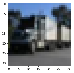
tensor(9) truck
Let's define a CNN:
import torch.nn as nn
import torch.nn.functional as F

class Net(nn.Module):
    def __init__(self):
        super(Net, self).__init__()
        self.conv1 = nn.Conv2d(3, 6, 5)
        self.pool = nn.MaxPool2d(2, 2)
        self.conv2 = nn.Conv2d(6, 16, 5)
        self.fc1 = nn.Linear(16 * 5 * 5, 120)
        self.fc2 = nn.Linear(120, 84)
        self.fc3 = nn.Linear(84, 10)

    def forward(self, x):
        x = self.pool(F.relu(self.conv1(x)))
        x = self.pool(F.relu(self.conv2(x)))
        x = x.view(-1, 16 * 5 * 5)
        x = F.relu(self.fc1(x))
        x = F.relu(self.fc2(x))
        x = self.fc3(x)
        return x

net = Net()
We can move it to GPU:
device = torch.device("cuda:1" if torch.cuda.is_available() else "cpu")
net.to(device)
Net(
(conv1): Conv2d(3, 6, kernel_size=(5, 5), stride=(1, 1))
(pool): MaxPool2d(kernel_size=2, stride=2, padding=0, dilation=1, ceil_mode=False)
(conv2): Conv2d(6, 16, kernel_size=(5, 5), stride=(1, 1))
(fc1): Linear(in_features=400, out_features=120, bias=True)
(fc2): Linear(in_features=120, out_features=84, bias=True)
(fc3): Linear(in_features=84, out_features=10, bias=True)
)
Define a loss function and optimizer:
import torch.optim as optim

criterion = nn.CrossEntropyLoss()
optimizer = optim.SGD(net.parameters(), lr=0.001, momentum=0.9)
Training:
for epoch in range(3):

    sum_loss = 0.0
    max_show = 3000
    for i, data in enumerate(trainloader, 0):
        # get the inputs
        inputs, labels = data

        # send to GPU
        inputs, labels = inputs.to(device), labels.to(device)

        # zero the parameter gradients
        optimizer.zero_grad()

        # forward + backward + optimize
        outputs = net(inputs)
        loss = criterion(outputs, labels)
        loss.backward()
        optimizer.step()

        # print statistics
        sum_loss += loss.item()
        if (i+1) % max_show == 0:    # print every 3000 mini-batches
            print('[%d, %5d] loss: %.3f' %
                  ((epoch+1), (i+1), (sum_loss/max_show)))
            sum_loss = 0.0

print('Finished Training')
[1, 3000] loss: 0.774
[1, 6000] loss: 0.807
[1, 9000] loss: 0.832
[1, 12000] loss: 0.844
[2, 3000] loss: 0.722
[2, 6000] loss: 0.791
[2, 9000] loss: 0.804
[2, 12000] loss: 0.820
[3, 3000] loss: 0.711
[3, 6000] loss: 0.761
[3, 9000] loss: 0.776
[3, 12000] loss: 0.786
Finished Training
Test our trained model on test data:
sum_correct = 0
sum_test = 0

with torch.no_grad():
    for data in testloader:
        images, labels = data
        images, labels = images.to(device), labels.to(device)

        outputs = net(images) # 4x10
        _, predicted = torch.max(outputs.data, 1) # (max_value, index)

        sum_correct += (predicted==labels).sum().item()
        sum_test += labels.size(0)

    print("Accuracy on 10000 test images: %.3f %%" % (100*sum_correct/sum_test))
Accuracy on 10000 test images: 63.140 %
1.5. Data Parallelism
We will learn how to use multiple GPUs using DataParallel.
DataParallel splits your data automatically and sends job orders to multiple models on several GPUs. After each model finishes their job, DataParallel collects and merges the results before returning it to you.
Please note that: just calling my_tensor.to(device) returns a new copy of my_tensor on GPU instead of rewriting my_tensor. You need to assign it to a new tensor and use that tensor on the GPU.
It is easy to make your model run parallelly using DataParallel:
model = nn.DataParallel(model)
Let's see an example.
### Imports and parameters
import torch
import torch.nn as nn
from torch.utils.data import Dataset, DataLoader

input_size = 5
output_size = 2

batch_size = 30
data_size = 100

device = torch.device("cuda:0")

### Dummy dataset
class RandomDataset(Dataset):

    def __init__(self, size, length):
        self.len = length
        self.data = torch.randn(length, size)

    def __getitem__(self, index):
        return self.data[index]

    def __len__(self):
        return self.len

### Simple model
class Model(nn.Module):

    def __init__(self, input_size, output_size):
        super(Model, self).__init__()
        self.fc = nn.Linear(input_size, output_size)

    def forward(self, input):
        output = self.fc(input)
        print("\tInside the model: input size",input.size(),"output size",output.size())

        return output

### Create model and dataparallel
model = Model(input_size, output_size)
if torch.cuda.device_count() > 1:
    print(torch.cuda.device_count(),"GPUs are found!")
model = nn.DataParallel(model)
model.to(device)

### Run the model
rand_loader = DataLoader(dataset=RandomDataset(input_size, data_size),
                        batch_size=batch_size, shuffle=True)
for data in rand_loader:
    input = data.to(device)
    output = model(input)
    print("Total: Input size",input.size(),"output size",output.size())
2 GPUs are found!
Inside the model: input size torch.Size([15, 5]) output size torch.Size([15, 2])
Inside the model: input size torch.Size([15, 5]) output size torch.Size([15, 2])
Total: Input size torch.Size([30, 5]) output size torch.Size([30, 2])
Inside the model: input size torch.Size([15, 5]) output size torch.Size([15, 2])
Inside the model: input size torch.Size([15, 5]) output size torch.Size([15, 2])
Total: Input size torch.Size([30, 5]) output size torch.Size([30, 2])
Inside the model: input size torch.Size([15, 5]) output size torch.Size([15, 2])
Inside the model: input size torch.Size([15, 5]) output size torch.Size([15, 2])
Total: Input size torch.Size([30, 5]) output size torch.Size([30, 2])
Inside the model: input size torch.Size([5, 5]) output size torch.Size([5, 2])
Inside the model: input size torch.Size([5, 5]) output size torch.Size([5, 2])
Total: Input size torch.Size([10, 5]) output size torch.Size([10, 2])
2. 数据装载和处理
PyTorch provides many tools to make data loading easy and hopefully, to make your code more readable.
For this tutorial, we should install two packages:
scikit-image: Image io and transformspandas: Easier csv parsing
We have prepared a pose estimation database in ./data/faces. There are some human faces and their landmark points stored in .csv.
Let's read the CSV and get the annotations in an (N,2) array:
import pandas as pd
from skimage import io
import matplotlib.pyplot as plt

landmarks_list = pd.read_csv('data/faces/face_landmarks.csv')
'''
image_name,part_0_x,part_0_y,part_1_x,part_1_y,part_2_x, ... ,part_67_x,part_67_y
0805personali01.jpg,27,83,27,98, ... 84,134
1084239450_e76e00b7e7.jpg,70,236,71,257, ... ,128,312
'''

n = 50
img_name = landmarks_list.iloc[n, 0]
landmarks = landmarks_list.iloc[n, 1:].values.astype('float').reshape(-1,2) # pandas dict -> values

def show_landmarks(image, landmarks):
    'Show image with landmarks.'
    plt.imshow(image)
    plt.scatter(landmarks[:,0],landmarks[:,1], s=10, marker=".", c="r")
    plt.pause(0.001) # pause a bit so that plots are updated

plt.figure()
img_path = "./data/faces/"+img_name
show_landmarks(io.imread(img_path), landmarks)
plt.show()

2.1. Dataset Class
torch.utils.data.Dataset is an abstract class representing a dataset. Our custom dataset should inherit Dataset and override the following methods:
__len__: so thatlen(dataset)returns the size of the dataset.__getitem__: so thatdataset[i]can used for indexing.
Demo:
from torch.utils.data import Dataset
import os
class FaceLandmarksDataset(Dataset):
'Face landmarks dataset.'
def __init__(self, CsvFile_path, dir_img, transform=None):
self.landmarks_list = pd.read_csv(CsvFile_path)
self.dir_img = dir_img
self.transform = transform
def __len__(self):
return len(self.landmarks_list)
def __getitem__(self, idx):
img_path = os.path.join(self.dir_img,
self.landmarks_list.iloc[idx, 0])
image = io.imread(img_path)
landmarks = self.landmarks_list.iloc[idx, 1:].values.astype("float").reshape(-1,2)
sample = {'image':image, 'landmarks': landmarks}
if self.transform:
sample = self.transform(sample)
return sample
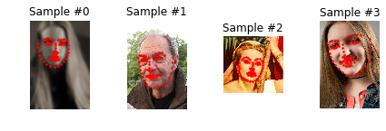
### Instantiate this class and show four images.
face_landmarks = FaceLandmarksDataset(CsvFile_path='./data/faces/face_landmarks.csv', dir_img='./data/faces/')
fig = plt.figure()
for i in range(len(face_landmarks)):
sample = face_landmarks[i]
print(i, sample['image'].shape, sample['landmarks'].shape)
ax = plt.subplot(1,4,i+1)
ax.set_title('Sample #{}'.format(i))
ax.axis('off')
ax.imshow(sample['image'])
ax.scatter(sample['landmarks'][:,0],sample['landmarks'][:,1], s=10, marker=".", c="r")
#show_landmarks(**sample)
if i == 3:
plt.tight_layout()
plt.show()
break
0 (324, 215, 3) (68, 2)
1 (500, 333, 3) (68, 2)
2 (250, 258, 3) (68, 2)
3 (434, 290, 3) (68, 2)
2.2. Transforms
We want to:
- randomly crop samples.
- rescale images.
- convert the numpy images to torch images (notice: swap axes).
We also want to write them as callable classes instead of simple functions:
from skimage import transform
import numpy as np

class Rescale():
    '''
    Rescale the image in a sample to a given size.

    Args:
        output_size (tuple or int): Desired output size. If int, the smaller image edge is matched to it
            and the aspect ratio remains the same.
    '''
    def __init__(self, output_size):
        assert isinstance(output_size, (int, tuple)) # ensure that output_size is an int or a tuple.
        self.output_size = output_size

    def __call__(self, sample):
        image, landmarks = sample['image'], sample['landmarks']

        h, w = image.shape[:2]
        if isinstance(self.output_size, int): # int: the length of the smaller edge
            if h > w:
                new_h, new_w = self.output_size * h / w, self.output_size
            else:
                new_h, new_w = self.output_size, self.output_size * w / h
        else:
            new_h, new_w = self.output_size
        new_h, new_w = int(new_h), int(new_w)

        image = transform.resize(image, (new_h, new_w))
        landmarks = landmarks * [new_w/w, new_h/h]

        return {'image':image, 'landmarks':landmarks}

class RandomCrop():
    '''
    Crop the image in a sample randomly.

    Args:
        output_size (tuple or int). If int, square crop is made.
    '''
    def __init__(self, output_size):
        assert isinstance(output_size, (int, tuple)) # ensure that output_size is an int or a tuple.
        self.output_size = output_size

    def __call__(self, sample):
        image, landmarks = sample['image'], sample['landmarks']

        h, w = image.shape[:2]
        if isinstance(self.output_size, int):
            new_h, new_w = self.output_size, self.output_size
        else:
            new_h, new_w = self.output_size

        start_h_idx = np.random.randint(0, h - new_h)
        start_w_idx = np.random.randint(0, w - new_w)

        image = image[start_h_idx: (start_h_idx+new_h),
                      start_w_idx: (start_w_idx+new_w)]
        landmarks = landmarks - [start_w_idx, start_h_idx]

        return {'image':image, 'landmarks':landmarks}

class ToTensor():
    '''
    Convert the ndarray image in a sample to a Tensor.
    Notice: swap color axis because:
        numpy image: H x W x C
        torch image: C X H X W
    '''
    def __call__(self, sample):
        image, landmarks = sample['image'], sample['landmarks']
        image = image.transpose((2, 0, 1))
        return {'image': torch.from_numpy(image),
                'landmarks': torch.from_numpy(landmarks)}
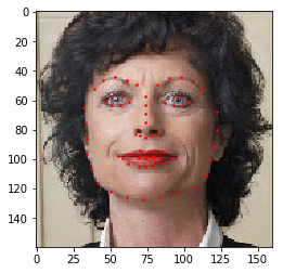
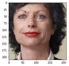
We now apply our transforms on an sample:
from torchvision import transforms

scale = Rescale(256) # the length of the smaller side is 256
crop = RandomCrop(210) # crop a 128x128 img
composed_trans = transforms.Compose([scale, crop])

fig = plt.figure()
plt.tight_layout()

sample = face_landmarks[65]
transformed_sample = composed_trans(sample)

show_landmarks(**sample)
show_landmarks(**transformed_sample)

plt.show()
2.3. Iterating through the Dataset
有了数据集,我们需要不断从中获取数据,用于训练或测试。
import torch

transformed_dataset = FaceLandmarksDataset(CsvFile_path='./data/faces/face_landmarks.csv',
                                           dir_img='./data/faces/',
                                           transform=transforms.Compose([
                                               Rescale(256),
                                               RandomCrop(210),
                                               ToTensor()
                                           ]))

for i in range(len(transformed_dataset)):
    sample = transformed_dataset[i]
    print(i, sample['image'].size(), sample['landmarks'].size())

    if i == 4:
        break
0 torch.Size([3, 210, 210]) torch.Size([68, 2])
1 torch.Size([3, 210, 210]) torch.Size([68, 2])
2 torch.Size([3, 210, 210]) torch.Size([68, 2])
3 torch.Size([3, 210, 210]) torch.Size([68, 2])
4 torch.Size([3, 210, 210]) torch.Size([68, 2])
However, we also want to:
- batch the data.
- shuffle the data.
- Load the data in parallel.
torch.utils.DataLoader is an iterator which provides all these features.
from torch.utils.data import DataLoader
from torchvision import utils

dataloader = DataLoader(transformed_dataset, batch_size=4,
                    shuffle=True, num_workers=0) # Windows may error when num_workers > 0

def show_landmarks_batch(sample_batch):
    'Show images with landmarks for a batch of samples.'
    image_batch, landmarks_batch = sample_batch['image'], sample_batch['landmarks']

    batch_size = len(image_batch)
    im_size = image_batch.size(2)

    grid = utils.make_grid(image_batch)
    plt.imshow(grid.numpy().transpose((1,2,0))) # Tensors -> ndarrays -> CxHxW to HxWxC

    for i in range(batch_size):
        plt.scatter(landmarks_batch[i,:,0].numpy()+im_size*i,
                    landmarks_batch[i,:,1].numpy(),
                    s=10, marker='.', c='r')
        plt.title('A batch from dataloader')

ite_batch = 3
for ite,sample_batch in enumerate(dataloader):
    print(sample_batch['image'].size(),
          sample_batch['landmarks'].size())
    if ite == ite_batch:
        plt.figure()
        show_landmarks_batch(sample_batch)
        plt.axis('off')
        plt.show()
        break
torch.Size([4, 3, 210, 210]) torch.Size([4, 68, 2])
torch.Size([4, 3, 210, 210]) torch.Size([4, 68, 2])
torch.Size([4, 3, 210, 210]) torch.Size([4, 68, 2])
torch.Size([4, 3, 210, 210]) torch.Size([4, 68, 2])

2.4. Torchvision
torchvision package provides some common datasets and transforms.
We might not even have to write custom classes. One of the more generic datasets available in torchvision is ImageFolder. It assumes that images are organized in the following way:
root/ants/xxx.png
root/ants/xxy.jpeg
root/ants/xxz.png
.
.
.
root/bees/123.jpg
root/bees/nsdf3.png
root/bees/asd932_.png
where ants and bees are class labels.
Besides, generic transforms in PIL.Image like RandomHorizontalFlip, Scale are also available.
import torch
from torchvision import transforms, datasets

data_transform = transforms.Compose([
    transforms.RandomSizedCrop(224),
    transforms.RandomHorizontalFlip(),
    transforms.ToTensor(),
    transforms.Normalize(mean=[0.485, 0.456, 0.406],
                        std = [0.229, 0.224, 0.225])
])

hymenoptera_dataset = datasets.ImageFolder(root='hymenoptera_data/train',
                                          transform=data_transform)

dataset_loader = torch.utils.data.DataLoader(hymenoptera_dataset,
                                            batch_size=4,shuffle=True,num_workers=0)
3. 温习和拓展:PyTorch好在哪
我们之前提到,PyTorch的核心功能可以归结为以下二者:
- A replacement for NumPy to use the power of GPUs.
- A deep learning research platform that provides maximum flexibility and speed.
即:
- 用GPU承载张量运算。
- 提供深度学习所需的其他功能。
我们可以阐释得更清楚:PyTorch provides:
- An n-dimensional Tensor, similar to numpy but can run on GPUs.
- Automatic differentiation for building and training neural networks.
原因如下:
- GPU能提供50倍甚至更多的运算加速。
- 现今深度学习方法仍然离不开BP方法,因此差分法求梯度是不可或缺的。其中自动差分技术是被广泛使用的。
3.1. 基本概念:Tensors and Autograd
Tensor在概念上和NumPy的array本质上是一致的,但Tensor的功能更全面:
Tensor携带着运算图(computational graph)和梯度信息,并且可以保持追踪状态;运算图上的节点就是Tensor,边缘(edges)是函数(functions)。Tensor可以使用GPU完成数值计算。
我们来看一个两层全连接网络的例子:
import torch

### Settings
dtype = torch.float32
device = torch.device("cuda:0")
learning_rate = 1e-6
total_ite = 500
N_batch, D_in, H, D_out = 64, 1000, 100, 10

### Creat random data set (Tensors)
x = torch.randn(N_batch, D_in, device=device, dtype=dtype)
y = torch.randn(N_batch, D_out, device=device, dtype=dtype)

### Initialize weight Tensors randomly
w1 = torch.randn(D_in, H, device=device, dtype=dtype, requires_grad=True)
w2 = torch.randn(H, D_out, device=device, dtype=dtype, requires_grad=True)

### Iterations
for ite in range(1,total_ite+1):

    y_pred = x.mm(w1).clamp(min=0).mm(w2) # clamp acts as relu function
    loss = (y_pred -y ).pow(2).sum()
    if ite % 100 == 0:
        print(ite, loss.item())

    loss.backward()

    # Manually update weights
    # Weights have requires_grad=True, but we don't need tracking.
    with torch.no_grad():

        w1 -= learning_rate * w1.grad
        w2 -= learning_rate * w2.grad

        # Maunally zero the gradients after updating weights
        w1.grad.zero_()
        w2.grad.zero_()
100 616.6424560546875
200 5.097920894622803
300 0.06861867755651474
400 0.0014389019925147295
500 0.0001344898482784629
TensorFlow和PyTorch最大的不同是:
- TensorFlow的运算图(computational graphs)是静态的(static):当定义好后,我们可以多次使用相同的运算图,只有输入数据可以不同。
- PyTorch的运算图是动态的(dynamic):每次前向传递(forward pass)时,运算图可以是全新的。
静态运算图可以进一步优化,因此效率比较高;但在一些场合比如反馈网络(recurrent network),更新动态运算图会更加简单。
我们在下下节会给一个例子。
还有一点不同:在TensorFlow中,参数更新是包含在运算图内的,而PyTorch反之。因此在PyTorch中我们应该停止梯度追逐。
3.2. 简化操作:nn Module
显然,上面的手动前向传导和参数迭代繁琐的。特别当网络复杂庞大时,参数是很难显式列举的。
PyTorch提供了一些模块来解决这些问题。
首先是简化网络定义。简单来说,nn包含了许多神经网络常用组件以及一些常用的损失函数。
定义好网络后,其中的参数会自动纳入学习参数(learnable parameters)列表内。
回到之前的例子:
import torch

### Settings
dtype = torch.float32
device = torch.device("cuda:0")
learning_rate = 1e-4 # bigger!
total_ite = 500
N_batch, D_in, H, D_out = 64, 1000, 100, 10

### Creat random data set (Tensors)
x = torch.randn(N_batch, D_in, device=device, dtype=dtype)
y = torch.randn(N_batch, D_out, device=device, dtype=dtype)

### Define network model by nn package
model = torch.nn.Sequential(
    torch.nn.Linear(D_in, H),
    torch.nn.ReLU(),
    torch.nn.Linear(H, D_out)
)
model = model.to(device)

### Define loss function by nn package
loss_fn = torch.nn.MSELoss(reduction='sum')

for ite in range(1, total_ite+1):

    y_pred = model(x)
    loss = loss_fn(y_pred, y)
    if ite % 100 == 0:
        print(ite, loss.item())

    model.zero_grad()
    loss.backward()

    # Manually update weights
    with torch.no_grad():

        for param in model.parameters():
            param -= learning_rate * param.grad
100 2.5298514366149902
200 0.04136687144637108
300 0.0011623052414506674
400 4.448959225555882e-05
500 2.1180185285629705e-06
其次是简化优化步骤。PyTorch提供了optim包,可以支持更加复杂的优化方法。
import torch

### Settings
dtype = torch.float32
device = torch.device("cuda:0")
learning_rate = 1e-4 # bigger!
total_ite = 500
N_batch, D_in, H, D_out = 64, 1000, 100, 10

### Creat random data set (Tensors)
x = torch.randn(N_batch, D_in, device=device, dtype=dtype)
y = torch.randn(N_batch, D_out, device=device, dtype=dtype)

### Define network model by nn package
model = torch.nn.Sequential(
    torch.nn.Linear(D_in, H),
    torch.nn.ReLU(),
    torch.nn.Linear(H, D_out)
)
model = model.to(device)

### Define loss function by nn package
loss_fn = torch.nn.MSELoss(reduction='sum')

### Define optimizer
optimizer = torch.optim.Adam(model.parameters(), lr=learning_rate)

for ite in range(1, total_ite+1):

    y_pred = model(x)
    loss = loss_fn(y_pred, y)
    if ite % 100 == 0:
        print(ite, loss.item())

    optimizer.zero_grad()
    loss.backward()

    # Update parameters
    optimizer.step()
100 65.00260925292969
200 1.0924508571624756
300 0.006899723317474127
400 5.2772647904930636e-05
500 1.6419755866081687e-07
nn包中提供的网络组件是很基本的。如果我们的网络很复杂,那么我们还可以自定义复杂网络:
import torch

class TwoLayerNet(torch.nn.Module):

    def __init__(self, D_in, H, D_out):

        super(TwoLayerNet, self).__init__()
        self.linear1 = torch.nn.Linear(D_in, H)
        self.linear2 = torch.nn.Linear(H, D_out)

    def forward(self, x):

        h_relu = self.linear1(x).clamp(min=0)
        y_pred = self.linear2(h_relu)
        return y_pred

### Settings
dtype = torch.float32
device = torch.device("cuda:0")
learning_rate = 1e-4 # bigger!
total_ite = 500
N_batch, D_in, H, D_out = 64, 1000, 100, 10

### Creat random data set (Tensors)
x = torch.randn(N_batch, D_in, device=device, dtype=dtype)
y = torch.randn(N_batch, D_out, device=device, dtype=dtype)

### Define network model by nn package
model = TwoLayerNet(D_in, H, D_out)
model = model.to(device)

### Define loss function by nn package
loss_fn = torch.nn.MSELoss(reduction='sum')

### Define optimizer
optimizer = torch.optim.Adam(model.parameters(), lr=learning_rate)

for ite in range(1, total_ite+1):

    y_pred = model(x)
    loss = loss_fn(y_pred, y)
    if ite % 100 == 0:
        print(ite, loss.item())

    optimizer.zero_grad()
    loss.backward()
    optimizer.step()
100 71.93133544921875
200 1.759734869003296
300 0.012220818549394608
400 0.0002741872740443796
500 1.9429817257332616e-05
3.3. 动态优势:Control Flow + Weight Sharing of PyTorch
在这一节,我们要举例介绍PyTorch的动态图优势。
首先,我们要搭建一个全连接网络。该网络的特点是:
- 每次前向传播时,隐藏层数目是随机的,可能是1,2,3或4;
- 隐藏层的参数是共享的。
import torch
import random

class DynamicNet(torch.nn.Module):

    def __init__(self, D_in, H, D_out):

        super(DynamicNet, self).__init__()
        self.input_linear = torch.nn.Linear(D_in, H)
        self.middle_linear = torch.nn.Linear(H, H)
        self.output_linear = torch.nn.Linear(H, D_out)

    def forward(self, x):

        h_relu = self.input_linear(x).clamp(min=0)
        rand_num = random.randint(0, 3)
        for _ in range(rand_num): # 1 layer, 2 layers, 3 layers or 4 layers
            h_relu = self.middle_linear(h_relu).clamp(min=0)
        y_pred = self.output_linear(h_relu)
        return y_pred, rand_num

### Settings
dtype = torch.float32
device = torch.device("cuda:0")
learning_rate = 1e-4
momentum = 0.9
total_ite = 500
N_batch, D_in, H, D_out = 64, 1000, 100, 10

### Creat random data set (Tensors)
x = torch.randn(N_batch, D_in, device=device, dtype=dtype)
y = torch.randn(N_batch, D_out, device=device, dtype=dtype)

### Define network model by nn package
model = DynamicNet(D_in, H, D_out)
model = model.to(device)

### Define loss function by nn package
loss_fn = torch.nn.MSELoss(reduction='sum')

### Define optimizer
optimizer = torch.optim.SGD(model.parameters(), lr=learning_rate, momentum=momentum)

for ite in range(1, total_ite+1):

    y_pred, rand_num = model(x)
    loss = loss_fn(y_pred, y)
    if ite % 100 == 0:
        print(ite, loss.item(), rand_num)

    optimizer.zero_grad()
    loss.backward()
    optimizer.step()
100 13.738285064697266 0
200 4.243963718414307 2
300 0.7942993640899658 1
400 0.43234169483184814 3
500 0.42137715220451355 2
4. 迁移学习(TRANSFER LEARNING)
假设我们要迁移一个卷积网络(convnet)。有两种主要方式:
- Finetune整个网络:迁移网络的所有参数都不是冻结的。
- 冻结迁移网络:只有新增的或后几层网络是可训练的。
我们先从数据装载和训练开始。
4.1. 装载数据
4.1.1. 构建数据装载器
我们的任务是:训练一个蚂蚁、蜜蜂分类器。每个类别分别有120张训练图片和75张测试图片。
显然,训练集是比较小的,因此迁移学习将是一个不错的选择。
数据下载地址:https://download.pytorch.org/tutorial/hymenoptera_data.zip
下载完毕后,文件夹hymenoptera_data放置在当前文件夹下。
import torch
from torchvision import datasets, transforms
import os

device = torch.device("cuda:1" if torch.cuda.is_available() else "cpu")

data_dir = "./hymenoptera_data"
data_transform = {
    'train': transforms.Compose([
        transforms.RandomResizedCrop(224),
        transforms.RandomHorizontalFlip(),
        transforms.ToTensor(),
        transforms.Normalize([0.485, 0.456, 0.406], [0.229, 0.224, 0.225])
    ]),
    'val': transforms.Compose([
        transforms.Resize(256),
        transforms.CenterCrop(224),
        transforms.ToTensor(),
        transforms.Normalize([0.485, 0.456, 0.406], [0.229, 0.224, 0.225])
    ])
}

image_datasets = {x: datasets.ImageFolder(os.path.join(data_dir, x),
                                          data_transform[x])
                  for x in ['train', 'val']}
dataloaders = {x: torch.utils.data.DataLoader(image_datasets[x],
                                              batch_size=4,
                                              shuffle=True,
                                              num_workers=4)
               for x in ['train', 'val']}

dataset_sizes = {x: len(image_datasets[x]) for x in ['train', 'val']}
class_names = image_datasets['train'].classes
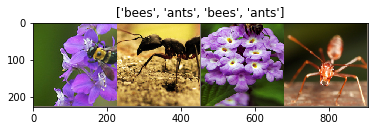
4.1.2. 展示一些训练样本
import numpy as np
import matplotlib.pyplot as plt
import torchvision

plt.ion() # interactive mode

def imshow(input, title=None):
    'Imshow for Tensors.'
    input = input.numpy().transpose((1,2,0))
    means = np.array([0.485, 0.456, 0.406])
    stds = np.array([0.229, 0.224, 0.225])
    input = input * stds + means
    input = np.clip(input, 0, 1)
    plt.imshow(input)
    if title is not None:
        plt.title(title)
    plt.pause(0.001) # pause a bit so that plots can be updated

inputs, classes = next(iter(dataloaders['train']))
input = torchvision.utils.make_grid(inputs)
imshow(input, title=[class_names[x] for x in classes])
4.2. 训练
在训练过程中,我们将会完成两个任务:
- 调整学习率:通过
torch.optim.lr_scheduler,基于epoches数来自行调整scheduler。 - 保存最佳模型。
import torch.optim as optim
from torch.optim import lr_scheduler
import time
import copy
from torchvision import models
import torch.nn as nn

def train_model(model, criterion, optimizer, scheduler, num_epochs=25):
    'Finetune model and return the best model.'
    time_start = time.time()

    # Init
    best_model = copy.deepcopy(model.state_dict())
    best_acc = 0.0

    # Train and eval epoch by epoch
    for epoch in range(num_epochs):

        for phase in ['train', 'val']:
            if phase == 'train':
                scheduler.step()
                model.train() # Set model to training mode
            else:
                model.eval() # Set model to evaluate mode

            # Run model
            running_loss = 0.0 # Init for accumulation
            running_corrects = 0

            for inputs, labels in dataloaders[phase]:
                # Move to GPU
                inputs = inputs.to(device)
                labels = labels.to(device)

                # Zero gradients
                optimizer.zero_grad()

                # Forward
                with torch.set_grad_enabled(phase == 'train'):
                    outputs = model(inputs)
                    loss = criterion(outputs, labels)
                    _, preds = torch.max(outputs, 1)

                    if phase == 'train':
                        loss.backward()
                        optimizer.step()

                # Accumulation
                running_loss += loss.item() * inputs.size(0)
                running_corrects += torch.sum(preds == labels.data)

            # Evaluation
            epoch_loss = running_loss / dataset_sizes[phase]
            epoch_acc = running_corrects.double() / dataset_sizes[phase]

            if phase == 'val' and epoch_acc > best_acc:
                best_acc = epoch_acc
                best_model = copy.deepcopy(model.state_dict())

            if ((epoch + 1) % 5 == 0) or (epoch == num_epochs):
                if phase == 'train':
                    print('Epoch {}/{}'.format(epoch+1, num_epochs))
                print('{:5s} loss: {:.3f} acc: {:.3f}'.format(phase, epoch_loss, epoch_acc))
                if phase == 'val':
                    print('')

    time_elapsed = time.time() - time_start
    print('Training complete in {:.0f}m {:.0f}s'.format((time_elapsed // 60),
                                                        (time_elapsed % 60)))
    print('Best val acc: {:.3f}'.format(best_acc))

    # Load best model
    model.load_state_dict(best_model)
    return model

### Finetune the convnet
model_ft = models.resnet18(pretrained=True) # Returns a model pre-trained on ImageNet
num_fc_in = model_ft.fc.in_features
model_ft.fc = nn.Linear(num_fc_in, 2)

model_ft = model_ft.to(device)
criterion = nn.CrossEntropyLoss()
optimizer_ft = optim.SGD(model_ft.parameters(), lr=0.001, momentum=0.9)
exp_lr_scheduler = lr_scheduler.StepLR(optimizer_ft, step_size=7, gamma=0.1) # Decay LR by a factor of 0.1 every 7 epochs
model_ft = train_model(model_ft, criterion, optimizer_ft, exp_lr_scheduler,
                       num_epochs=25)
Epoch 5/25
train loss: 0.348 acc: 0.857
val loss: 0.261 acc: 0.902
Epoch 10/25
train loss: 0.339 acc: 0.861
val loss: 0.193 acc: 0.928
Epoch 15/25
train loss: 0.285 acc: 0.885
val loss: 0.198 acc: 0.915
Epoch 20/25
train loss: 0.255 acc: 0.893
val loss: 0.177 acc: 0.922
Epoch 25/25
train loss: 0.250 acc: 0.893
val loss: 0.268 acc: 0.908
Training complete in 2m 41s
Best val acc: 0.928
以上有一些需要注意的:
-
torchvision.models中有大量网络模型,包括VGG,DenseNet,ResNet等。 -
进一步,我们还可以得到在ImageNet上预训练好的模型。只需要设置
pretrained=True即可得到,模型会下载、保存至torch.utils.model_zoo规定的路径下。 -
一些网络的训练和测试行为是不同的,例如存在BN的网络。因此需要调用
model.train()或model.eval()来切换。 -
所有的预训练模型都要求输入RGB图像(维度:
3xHxW)的长和宽不小于224,并且要经过正则化:mean = [0.485, 0.456, 0.406], std = [0.229, 0.224, 0.225]。一般是借助变换实现:
normalize = transforms.Normalize(mean=[0.485, 0.456, 0.406],
                                 std=[0.229, 0.224, 0.225])
Tensor.data()是已经被抛弃的方法,用于产生一个与原张量一样的张量,不篡改原张量的计算历史。
现在建议都用.detach()代替,更安全。
4.3. 冻结前几层
现在我们尝试:只finetune最后的FC层,前面所有层都冻结。方法其实很简单:
- 将预训练网络中所有参数的梯度追踪关闭,因为不参与迭代;
- 新建一个FC层,因为输出只有两类(蚂蚁和蜜蜂);
- 优化器只对FC层参数进行优化。
model_conv = torchvision.models.resnet18(pretrained=True)

for param in model_conv.parameters():
    param.requires_grad = False

num_fc_in = model_ft.fc.in_features
model_conv.fc = nn.Linear(num_fc_in, 2)

model_conv = model_conv.to(device)
criterion = nn.CrossEntropyLoss()
optimizer_conv = optim.SGD(model_conv.fc.parameters(), lr=0.001, momentum=0.9) # Notice params!!!
exp_lr_scheduler = lr_scheduler.StepLR(optimizer_conv, step_size=7, gamma=0.1)
model_conv = train_model(model_conv, criterion, optimizer_conv, exp_lr_scheduler,
                       num_epochs=25)
Epoch 5/25
train loss: 0.448 acc: 0.803
val loss: 0.240 acc: 0.902
Epoch 10/25
train loss: 0.304 acc: 0.881
val loss: 0.184 acc: 0.941
Epoch 15/25
train loss: 0.341 acc: 0.852
val loss: 0.185 acc: 0.941
Epoch 20/25
train loss: 0.412 acc: 0.820
val loss: 0.180 acc: 0.941
Epoch 25/25
train loss: 0.294 acc: 0.902
val loss: 0.187 acc: 0.941
Training complete in 2m 11s
Best val acc: 0.948
5. 保存和加载模型
我们需要掌握3个核心函数:
torch.save:将一个序列化的对象保存在本地磁盘上。序列化过程借助Python的pickle模块实现。无论是模型、张量还是词典型对象都可以保存。torch.load:使用pickle模块执行解序列化(deserialize)操作,将对象加载到内存中。torch.nn.Module.load_state_dict:借助一个解序列的state_dict,加载模型参数。
5.1. 什么是state_dict?
对于PyTorch,torch.nn.Module模型的参数都存储在model.parameters()中。
而state_dict是一个简单的Python字典对象,将模型的每一层映射为字典内的一个张量。
有可学习参数(learnable parameters)的网络层(如卷积层,线性映射层),以及被收录的缓冲器(如BN)可以保留在模型的state_dict中。
优化器对象torch.optim也有它的state_dict,保存了优化器的状态和超参数。
由于state_dict的本质是Python的字典,因此其读、存、写非常简单。
我们拿前面分类器的例子,看看该字典究竟存了什么。
import torch.nn as nn
import torch.nn.functional as F

# Define model
class model_class(nn.Module):
    def __init__(self):
        super(model_class, self).__init__()
        self.conv1 = nn.Conv2d(3, 6, 5)
        self.pool = nn.MaxPool2d(2, 2)
        self.conv2 = nn.Conv2d(6, 16, 5)
        self.fc1 = nn.Linear(16 * 5 * 5, 120)
        self.fc2 = nn.Linear(120, 84)
        self.fc3 = nn.Linear(84, 10)

    def forward(self, x):
        x = self.pool(F.relu(self.conv1(x)))
        x = self.pool(F.relu(self.conv2(x)))
        x = x.view(-1, 16 * 5 * 5)
        x = F.relu(self.fc1(x))
        x = F.relu(self.fc2(x))
        x = self.fc3(x)
        return x

# Initialize model
model = model_class()

# Initialize optimizer
optimizer = optim.SGD(model.parameters(), lr=0.001, momentum=0.9)

# Print model's state_dict
print("Model's state_dict:")
for param_tensor in model.state_dict():
    print(param_tensor, "\t", model.state_dict()[param_tensor].size())

# Print optimizer's state_dict
print("Optimizer's state_dict:")
for var_name in optimizer.state_dict():
    print(var_name, "\t", optimizer.state_dict()[var_name])
Model's state_dict:
conv1.weight torch.Size([6, 3, 5, 5])
conv1.bias torch.Size([6])
conv2.weight torch.Size([16, 6, 5, 5])
conv2.bias torch.Size([16])
fc1.weight torch.Size([120, 400])
fc1.bias torch.Size([120])
fc2.weight torch.Size([84, 120])
fc2.bias torch.Size([84])
fc3.weight torch.Size([10, 84])
fc3.bias torch.Size([10])
Optimizer's state_dict:
state {}
param_groups [{'lr': 0.001, 'momentum': 0.9, 'dampening': 0, 'weight_decay': 0, 'nesterov': False, 'params': [1831247242080, 1831247241936, 1831247242296, 1831247241864, 1831247242800, 1831247243232, 1831247242872, 1831247242584, 1831247243160, 1831247242656]}]
5.2. 保存和加载模型
5.2.1. 保存和加载state_dict(推荐)
torch.save(model.state_dict(), PATH) # Save

### Load
model.load_state_dict(torch.load(PATH))
model.eval()
值得注意的有两点:
- 加载完如果要测试,请务必设置为
eval模式。因为网络中可能存在dropout和BN等结构。若遗漏,那么结果可能不稳定。 - 不能直接通过
model.load_state_dict(PATH)进行加载,而需要先借助torch.load解序列。因为.load_state_dict函数的输入必须是一个字典对象。
5.2.2. 保存和加载整个模型
上面的方法只保存了参数数据,并没有保存结构信息。下面的方法很直接,保存所有信息:
torch.save(model, PATH) # Save

model = torch.load(PATH)
model.eval() # Load
缺点:torch.save直接对整个模型序列化存储,要求该模型数据必须是一些特定的类(specific classes)和字典结构。
在应用过程中,代码可能出错。
上述两种方法通常存为.pt或.pth文件。
5.3. 保存和加载特定节点的模型
首先提一下:如果为了保存后继续训练,可以把优化器的状态也保存备用。
### Save
torch.save({
    'epoch': epoch,
    'model_state_dict': model.state_dict(),
    'optimizer_state_dict': optimizer.state_dict(),
    'loss': loss
}, PATH)

### Load
model = model_class()
optimizer = optimizer_class()

checkpoint = torch.load(PATH) # just a dict
model.load_state_dict(checkpoint['model_state_dict'])
optimizer.load_state_dict(checkpoint['optimizer_state_dict'])
epoch = checkpoint['epoch']
loss = checkpoint['loss']

model.eval()
# - or -
model.train()
其实很好理解:无非是又创建了一个大字典,把state_dict作为小字典存于其中。大字典中还包含其他有用的信息。
通常存为.tar文件。
5.4. 在一个文件中保存多个模型
当我们保存如GAN模型等时,我们常常会有多个torch.nn.Modules对象。保存很简单:
### Save
torch.save({
            'modelA_state_dict': modelA.state_dict(),
            'modelB_state_dict': modelB.state_dict(),
            'optimizerA_state_dict': optimizerA.state_dict(),
            'optimizerB_state_dict': optimizerB.state_dict(),
            ...
            }, PATH)

### Load
modelA = ModelAClass(*args, **kwargs)
modelB = ModelBClass(*args, **kwargs)
optimizerA = TheOptimizerAClass(*args, **kwargs)
optimizerB = TheOptimizerBClass(*args, **kwargs)

checkpoint = torch.load(PATH)
modelA.load_state_dict(checkpoint['modelA_state_dict'])
modelB.load_state_dict(checkpoint['modelB_state_dict'])
optimizerA.load_state_dict(checkpoint['optimizerA_state_dict'])
optimizerB.load_state_dict(checkpoint['optimizerB_state_dict'])

modelA.eval()
modelB.eval()
# - or -
modelA.train()
modelB.train()
5.5. 转移部分参数
如果源网络和目标网络的参数不完全一致(或多或少key不同),那么可以设置strict=False:
model.load_state_dict(torch.load(PATH), strict=False)
此时,不匹配的key会自动被忽略。
如果只是名字不同,我们还可以直接修改state_dict!
5.6. 在不同设备上存储/读取
5.6.1. 在GPU和CPU之间
torch.save(model.state_dict(), PATH) # Save

model = TheModelClass(*args, **kwargs)

# Save on GPU, load on CPU
device = torch.device('cpu')
model.load_state_dict(torch.load(PATH, map_location=device))

# GPU, GPU
device = torch.device("cuda")
model.load_state_dict(torch.load(PATH))
model.to(device)

# Save on CPU, load on GPU
device = torch.device("cuda")
model.load_state_dict(torch.load(PATH, map_location="cuda:0")) # Choose whatever GPU device number you want
model.to(device)
总结:
- 只要设备不同,就需要设置
torch.load的参数map_location来完成映射。 - 如果模型要在GPU上跑,一定要将模型的参数转化为CUDA张量,就地更改。
- 输入数据也要转移到GPU上。但对张量而言,
tensor.to(device)并非就地更改,而是创建新的张量。因此一定要赋值:new_t = tensor.to(torch.device('cuda'))
5.6.2. 保存torch.nn.DataParallel模型
torch.save(model.module.state_dict(), PATH) # Save
torch.nn.DataParallel是一个模型装饰器(model wrapper),可以运行并行GPU运算。
我们只需要保存model.module.state_dict(),就可以将其加载到任意装置。
6. 究竟什么是torch.nn?
PyTorch提供了精美的模块和类来帮助我们构建神经网络,如torch.nn,torch.optim,Dataset及DataLoader。
在这一章,我们会从MNIST开始,一步步讲解这些模块和类的作用。这一章可以作为前面所学的回顾。
6.1. MNIST数据准备
首先我们用pathlib标准库定义下载路径;然后我们从这里用requests库下载文件放到路径下。
这里说一下以前的做法:
if not os.path.exists(directory):
    os.makedirs(directory)
这样做实际上是危险的,因为在os.path.exists()和os.makedirs()之间的时间内可能会出现目录被创建。
Python 3.5+提供了更加安全的pathlib的mkdir:
from pathlib import Path
path_data = Path("data")
path_mnist = path_data / "mnist"
path_mnist.mkdir(parents=True, exist_ok=True) # 若父目录不存在,则创建之;若目录已存在,则不创建且不报错。

import requests
url = "http://deeplearning.net/data/mnist/"
filename = "mnist.pkl.gz"
if not (path_mnist / filename).exists():
        content = requests.get(url + filename).content
        (path_mnist / filename).open("wb").write(content)
该数据集是NumPy数组,但以pickle格式存储(我们已经知道这是序列化后的)。因此我们需要特殊的读取方式:
- 通过
gzip.open读取压缩包。 - 通过
pickle.load()解序列。
import pickle
import gzip

with gzip.open((path_mnist / filename).as_posix(), "rb") as f:
        ((x_train, y_train), (x_valid, y_valid), _) = pickle.load(f, encoding="latin-1")
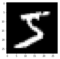
每个图像都是\(28 \times 28\)的,被拉伸为784维向量。如果需要展示图片,那么我们要先reshape:
from matplotlib import pyplot
import numpy as np

pyplot.imshow(x_train[0].reshape((28, 28)), cmap='gray')
print(x_train.shape)
(50000, 784)
为了进一步在GPU上运算,我们将数据转移(实际上是新建)至GPU:
import torch
x_train, y_train, x_valid, y_valid = map(
    torch.tensor, (x_train, y_train, x_valid, y_valid)
)
print(x_train.shape, y_train.shape)
print(x_valid.shape, y_valid.shape)
torch.Size([50000, 784]) torch.Size([50000])
torch.Size([10000, 784]) torch.Size([10000])
6.2. 用PyTorch(无torch.nn)实现一个神经网络
我们的模型是线性模型。
首先,我们要用Xavier初始化方法创建模型的变量:
import math

weights = torch.randn(784, 10)/ math.sqrt(784)
weights.requires_grad_()
bias = torch.zeros(10, requires_grad=True)
其次,我们要定义一些简单的函数:
def log_softmax(x):
    return x - x.exp().sum(-1).log().unsqueeze(-1)

def model(xb):
    return log_softmax(xb @ weights + bias) # @ stands for dot product operation
插一句:在多分类问题中,我们常用softmax函数。但在PyTorch中,对数用得更多。
然后,我们按照batch_size = 64完成一次前向传播:
bs = 64
xb = x_train[0:bs]
preds = model(xb)
print(preds[0], preds.shape)
tensor([-2.9072, -2.0663, -3.1907, -2.5540, -1.8701, -1.6411, -2.5566, -2.3751,
-2.1952, -2.6590], grad_fn=
需要注意到,preds不仅包含Tensor的值,还包含一个梯度函数。
此时我们再用负对数似然(negative log-likelihood)作为损失函数:
def nll(input, target):
    return -input[range(target.shape[0]), target].mean()

loss_func = nll

# e.g.
yb = y_train[0:bs]
print(loss_func(preds, yb))
tensor(2.3465, grad_fn=
还需要评估我们的预测结果(准确率):
def accuracy(out, yb):
    preds = torch.argmax(out, dim=1)
    return (preds == yb).float().mean()

print(accuracy(preds, yb))
tensor(0.1406)
下一步,我们利用循环迭代更新参数。注意,参数梯度是用PyTorch的自动差分计算得到的,而非手工计算。
from IPython.core.debugger import set_trace

lr = 0.5
epochs = 2

n = x_train.shape[0]

for epoch in range(epochs):
    for i in range((n - 1) // bs + 1):
        # set_trace()
        start_i = i * bs
        end_i = start_i + bs
        xb = x_train[start_i: end_i]
        yb = y_train[start_i: end_i]

        pred = model(xb)
        loss = loss_func(pred, yb)

        loss.backward()
        with torch.no_grad():
            weights -= weights.grad * lr
            bias -= bias.grad * lr

            weights.grad.zero_()
            bias.grad.zero_()

# Test
pred = model(xb)
print(loss_func(pred, yb), accuracy(pred, yb))
tensor(0.0852, grad_fn=
在训练集上的准确率达到了100!只是一个简单的非线性激活的线性网络。
其中要说明的是:通过设置set_trace(),我们可以使用标准的Python调试器(debugger)来检查每一步多个变量的值。
6.3. 使用torch.nn.functional提供的函数
现在,我们使用torch.nn.functional。该模块提供许多损失函数和激活函数(如下面的交叉熵),甚至还有一些网络模块(如池化函数)。
import torch.nn.functional as F

loss_func = F.cross_entropy

def model(xb):
    return xb @ weights + bias

pred = model(xb)
print(loss_func(pred, yb), accuracy(pred, yb))
tensor(0.0852, grad_fn=
可以看到,该损失结果和我们在上一节计算的是一致的。
6.4. 使用nn.Module提供的神经网络类
我们不希望列举所有的可学习参数,这样会显得非常笨拙。
PyTorch提供了nn.Module类来构建我们的神经网络。我们只需要继承该类的同时新建我们自己的网络类。
此时,我们的网络类就会将可学习参数承载,追踪梯度变化,并且具有.parameters()和.zero_grad()等有用的属性和方法。
注意第一个M是大写。
from torch import nn

class Mnist_Logistic(nn.Module):

    def __init__(self):
        super().__init__()
        self.weights = nn.Parameter(torch.randn(784, 10)/ math.sqrt(784))
        self.bias = nn.Parameter(torch.zeros(10))

    def forward(self, xb):
        return xb @ self.weights + self.bias

model = Mnist_Logistic()
其中要说明nn.Parameter。首先,Parameters是Tensor的子类;当在Module中出现时,该张量会被认为是模型的参数,从而被自动加入参数列表中,可以通过parameters()迭代器等方式获取。
现在,我们可以像调用函数一样直接调用nn.Module的对象,本质是自动调用forward方法:
pred = model(xb)
print(loss_func(pred, yb))
tensor(2.2320, grad_fn=
并且,参数更迭变得更简单,因为参数被收集在方法model.parameters()内。我们还可以利用model.zero_grad()方法:
with torch.no_grad():

    for p in model.parameters():
        p -= p.grad * lr

    model.zero_grad()
现在,我们将其放在一个函数内,完成2个epoch的迭代:
def fit():
    for epoch in range(epochs):
        for i in range((n - 1) // bs + 1):
            start_i = i * bs
            end_i = start_i + bs
            xb = x_train[start_i: end_i]
            yb = y_train[start_i: end_i]

            pred = model(xb)
            loss = loss_func(pred, yb)

            loss.backward()
            with torch.no_grad():
                for p in model.parameters():
                    p -= p.grad * lr

                model.zero_grad()

fit()

pred = model(xb)
print(loss_func(pred, yb))
tensor(0.0805, grad_fn=
6.5. 使用nn.Linear简化函数定义
class Mnist_Logistic(nn.Module):

    def __init__(self):
        super().__init__()
        self.lin = nn.Linear(784, 10)

    def forward(self, xb):
        return self.lin(xb)

model = Mnist_Logistic()

fit()

pred = model(xb)
print(loss_func(pred, yb))
tensor(0.0811, grad_fn=
6.6. 使用optim简化优化定义
我们有时会用到更复杂的优化器,此时torch.optim就提供了更多的选择。
from torch import optim

model = Mnist_Logistic()
opt = optim.SGD(model.parameters(), lr=lr)

pred = model(xb)
print(loss_func(pred, yb))

for epoch in range(epochs):
    for i in range((n - 1) // bs + 1):
        start_i = i * bs
        end_i = start_i + bs
        xb = x_train[start_i:end_i]
        yb = y_train[start_i:end_i]

        pred = model(xb)
        loss = loss_func(pred, yb)

        loss.backward()

        opt.step() # replace the loop for updating parameters
        opt.zero_grad()

pred = model(xb)
print(loss_func(pred, yb))
tensor(2.3233, grad_fn=
tensor(0.0832, grad_fn=
6.7. 使用Dataset简化数据获取
只要有__len__函数和一个__getitem__函数,任意对象都可以作为一个数据集(Dataset)。
PyTorch提供了TensorDataset函数。我们的数据集将被其装饰为一个新的张量TensorDataset,可以迭代,也可以在其第一个维度上切片(slice)。
在该例中,x_train和y_train还可以合二为一,这样索引会更加简单(一行足矣):
from torch.utils.data import TensorDataset

train_ds = TensorDataset(x_train, y_train)
此时训练变得更加轻巧:
model = Mnist_Logistic()
opt = optim.SGD(model.parameters(), lr=lr)

pred = model(xb)
print(loss_func(pred, yb))

for epoch in range(epochs):
    for i in range((n - 1) // bs + 1):
        start_i = i * bs
        end_i = start_i + bs
        xb, yb = train_ds[start_i:end_i]

        pred = model(xb)
        loss = loss_func(pred, yb)

        loss.backward()

        opt.step() # replace the loop for updating parameters
        opt.zero_grad()

pred = model(xb)
print(loss_func(pred, yb))
tensor(2.3649, grad_fn=
tensor(0.0819, grad_fn=
6.8. 使用DataLoader管理batch
我们还想扔掉batch的烦人的索引!此时,我们可以将Dataset进一步抽象为DataLoader:
from torch.utils.data import DataLoader

train_ds = TensorDataset(x_train, y_train)
train_dl = DataLoader(train_ds, batch_size=bs)

model = Mnist_Logistic()
opt = optim.SGD(model.parameters(), lr=lr)

pred = model(xb)
print(loss_func(pred, yb))

for epoch in range(epochs):
    for xb, yb in train_dl:

        pred = model(xb)
        loss = loss_func(pred, yb)

        loss.backward()

        opt.step() # replace the loop for updating parameters
        opt.zero_grad()

pred = model(xb)
print(loss_func(pred, yb))
tensor(2.2478, grad_fn=
tensor(0.0803, grad_fn=
6.9. 加入验证集(validation)及打乱训练集
train_ds = TensorDataset(x_train, y_train)
train_dl = DataLoader(train_ds, batch_size=bs, shuffle=True)

valid_ds = TensorDataset(x_valid, y_valid)
注意:我们需要在训练前调用model.train(),在测试前调用model.eval()。因为有一些特殊的结构如nn.BatchNorm2d和nn.Dropout在训练和测试时的表现是很不一样的。
model = Mnist_Logistic()
opt = optim.SGD(model.parameters(), lr=lr)

pred = model(xb)
print(loss_func(pred, yb))

for epoch in range(epochs):

    model.train()
    for xb, yb in train_dl:

        pred = model(xb)
        loss = loss_func(pred, yb)

        loss.backward()

        opt.step() # replace the loop for updating parameters
        opt.zero_grad()

    model.eval()
    with torch.no_grad():
        xb, yb = valid_ds[:]
        valid_pred = model(xb)
        valid_loss = loss_func(valid_pred, yb)

    print(epoch, valid_loss)
tensor(2.3226, grad_fn=
0 tensor(0.5259)
1 tensor(0.2907)
6.10. 简化为3行语句
上述过程一共分为3步:
- 得到
Dataset或DataLoader; - 建立模型
model和优化器opt; - 训练模型。
我们分别写为3个大函数,若干个小函数和类:
import numpy as np

def get_data(x_train, y_train, bs):
    # Returns training dataloader and a validation dataset.
    train_ds = TensorDataset(x_train, y_train)
    train_dl = DataLoader(train_ds, batch_size=bs, shuffle=True)

    valid_ds = TensorDataset(x_valid, y_valid)

    return train_dl, valid_ds

class Mnist_Logistic(nn.Module):
    # Defines our model.
    def __init__(self):
        super().__init__()
        self.lin = nn.Linear(784, 10)

    def forward(self, xb):
        return self.lin(xb)

def get_model():
    # Returns a model and optimizer.
    model = Mnist_Logistic()
    opt = optim.SGD(model.parameters(), lr=lr)
    return model, opt

loss_func = F.cross_entropy

def fit(epochs, model, loss_func, opt, train_dl, valid_ds):
    # Defines the training process
    for epoch in range(epochs):
        model.train()
        for xb, yb in train_dl:
            pred = model(xb)
            loss = loss_func(pred, yb)
            loss.backward()
            opt.step() # replace the loop for updating parameters
            opt.zero_grad()

        model.eval()
        with torch.no_grad():
            xb, yb = valid_ds[:]
            valid_pred = model(xb)
            valid_loss = loss_func(valid_pred, yb)

            print(epoch, valid_loss)
三句话完成!
train_dl, valid_ds = get_data(x_train, y_train, bs)

model, opt = get_model()

fit(epochs, model, loss_func, opt, train_dl, valid_ds)
0 tensor(0.3271)
1 tensor(0.2750)
6.11. 升级:CNN
此时,nn.Module提供的模块将会大放异彩:
class Mnist_CNN(nn.Module):
    # Defines a 3-layers CNN.
    def __init__(self):
        super().__init__()
        self.conv1 = nn.Conv2d(1, 16, kernel_size=3, stride=2, padding=1)
        self.conv2 = nn.Conv2d(16, 16, kernel_size=3, stride=2, padding=1)
        self.conv3 = nn.Conv2d(16, 10, kernel_size=3, stride=2, padding=1)

    def forward(self, xb):
        xb = xb.view(-1, 1, 28, 28) # Batch_size * 1 * 28 * 28
        xb = F.relu(self.conv1(xb)) #
        xb = F.relu(self.conv2(xb))
        xb = F.relu(self.conv3(xb))
        xb = F.avg_pool2d(xb, 4)
        xb = xb.view(-1, xb.size(1))
        return xb

def get_model():
    # Returns a model and optimizer.
    model = Mnist_CNN()
    opt = optim.SGD(model.parameters(), lr=0.1, momentum=0.9)
    return model, opt
现在开跑!
model, opt = get_model()

fit(epochs, model, loss_func, opt, train_dl, valid_ds)
0 tensor(0.3839)
1 tensor(0.2570)
6.12. 更简单地创建网络:nn.Sequential
如果我们的网络是流水线,那么nn.Sequential是一种更简单的创建方式。
其中的view函数并不是nn.Sequential可使用的。我们应该按以下方式改装:
class Lambda(nn.Module):
    def __init__(self, func):
        super().__init__()
        self.func = func

    def forward(self, x):
        return self.func(x)


def preprocess(x):
    return x.view(-1, 1, 28, 28)
也可以用匿名函数:
lambda x: x.view(-1, 1, 28, 28)
<function main.
那么网络可以这么写:
model = nn.Sequential(
    Lambda(preprocess),
    nn.Conv2d(1, 16, kernel_size=3, stride=2, padding=1),
    nn.ReLU(),
    nn.Conv2d(16, 16, kernel_size=3, stride=2, padding=1),
    nn.ReLU(),
    nn.Conv2d(16, 10, kernel_size=3, stride=2, padding=1),
    nn.ReLU(),
    nn.AvgPool2d(4),
    Lambda(lambda x: x.view(x.size(0), -1)),
)

opt = optim.SGD(model.parameters(), lr=0.1, momentum=0.9)

fit(epochs, model, loss_func, opt, train_dl, valid_ds)
0 tensor(0.3162)
1 tensor(0.2278)
6.13. 数据预处理
我们的模型鲁棒性很差,原因在两点:
- 输入必须是 \(28x28\)的向量或图像,因为
preprocess过程严格被定义。 - 最后的池化操作\(4x4\)的,因为池化函数的尺寸定义为4。
为了将CNN用于更广泛的场景,我们解除这两个封印。具体而言,我们加入了预处理函数(可根据需求修改),同时将nn.AvgPool2d改为nn.AdaptiveAvgPool2d(可规定输出尺寸而不是操作尺寸)。
详情参见原教程。
6.14. 使用GPU!
首先查看是否可以用GPU:
print(torch.cuda.is_available())
True
然后创建一个设备对象:
dev = torch.device("cuda:1") if torch.cuda.is_available() else torch.device("cpu")
在上一节中,我们可以在数据预处理函数中,将数据搬到dev上。然后我们再将model也搬到dev上。
我们改造原来的方法:
def get_data(x_train, y_train, bs):
    # Returns training dataloader and a validation dataset.
    train_ds = TensorDataset(x_train, y_train)
    train_dl = DataLoader(train_ds, batch_size=bs, shuffle=True)

    valid_ds = TensorDataset(x_valid, y_valid)

    return train_dl, valid_ds

class Mnist_Logistic(nn.Module):
    # Defines our model.
    def __init__(self):
        super().__init__()
        self.lin = nn.Linear(784, 10)

    def forward(self, xb):
        return self.lin(xb)

def get_model():
    # Returns a model and optimizer.
    model = Mnist_Logistic()
    model.to(dev)
    opt = optim.SGD(model.parameters(), lr=lr)
    return model, opt

loss_func = F.cross_entropy

def fit(epochs, model, loss_func, opt, train_dl, valid_ds):
    # Defines the training process
    for epoch in range(epochs):
        model.train()
        for xb, yb in train_dl:
            xb, yb = xb.to(dev), yb.to(dev)
            pred = model(xb)
            loss = loss_func(pred, yb)
            loss.backward()
            opt.step() # replace the loop for updating parameters
            opt.zero_grad()

        model.eval()
        with torch.no_grad():
            xb, yb = valid_ds[:]
            xb, yb = xb.to(dev), yb.to(dev)
            valid_pred = model(xb)
            valid_loss = loss_func(valid_pred, yb)

            print(epoch, valid_loss)

train_dl, valid_ds = get_data(x_train, y_train, bs)

model, opt = get_model()

fit(epochs, model, loss_func, opt, train_dl, valid_ds)
0 tensor(0.4048, device='cuda:1')
1 tensor(0.3062, device='cuda:1')

 浙公网安备 33010602011771号