python实现MICD分类器

from sklearn import datasets
import matplotlib.pyplot as plt
import numpy as np
from sklearn.model_selection import train_test_split


# MICD分类器
# 只能分辨训练集中存在的类别
class MICDClassifier:
    def __init__(self):
        self.center_dict = {}  # 分类中心点，以类别标签为键   label: center_point(list)
        self.sigma = {}  # 各类别样本的协方差矩阵，以类别标签为键
        self.sigma_I = {}  # 各类别样本协方差矩阵的逆，以类别标签为键
        self.feature_number = 0  # 特征维度
        self.train_state = False  # 训练状态，True为训练完成，False表示还没训练过

    # 特征白化，返回白化后的矩阵（numpy数组格式）
    # 参数为numpy格式的数组，其格式为数学上的矩阵的转置
    @staticmethod
    def whitening(feature_x):
        new_feature_x = np.asmatrix(feature_x).T
        sigma_x = np.cov(new_feature_x)
        eig_x = np.linalg.eig(sigma_x)  # 计算协方差矩阵sigma_x的特征值和特征向量
        diag_x = np.diag(eig_x[0])
        W = np.dot(np.power(np.asmatrix(diag_x).I, 0.5), eig_x[1].T)  # 记得eig_x[1]要转置！因为它是所求特征向量矩阵的转置
        return np.dot(W, new_feature_x).T.A  # 将矩阵转换为numpy的风格

    # 根据传入的样本集（特征+标签）来训练MICD分类器，
    # 其中每一个特征要求是行向量，标签也是行向量（为了与numpy array的格式对齐）
    # 函数将输入的标签数组转换为字典
    # 训练结果是记住样本中心点，以及根据样本计算特征的协方差矩阵
    def train(self, feature_set, label_set):
        new_label_set = {key: value for key, value in enumerate(label_set)}  # 将标签集合转换为以下标为键的字典   index: label
        self.feature_number = len(feature_set[0])
        sample_num = len(label_set)  # 样本个数
        count = {}  # 计算每个类别的样本个数  label: count(int)
        # 计算每个类别的分类中心点
        for index in range(sample_num):
            if new_label_set[index] not in count.keys():
                count[new_label_set[index]] = 0
                self.sigma[new_label_set[index]] = [feature_set[index]]
            else:
                count[new_label_set[index]] += 1  # 计算对应标签的样本数
                self.sigma[new_label_set[index]].append(feature_set[index])
            if new_label_set[index] not in self.center_dict.keys():
                self.center_dict[new_label_set[index]] = feature_set[index]
            else:
                self.center_dict[new_label_set[index]] += feature_set[index]
        for _key_ in self.center_dict.keys():
            for _feature_ in range(self.feature_number):
                self.center_dict[_key_][_feature_] /= count[_key_]
        for _key_ in self.sigma.keys():
            self.sigma[_key_] = np.cov(np.asmatrix(self.sigma[_key_]).T)  # 根据样本计算特征的协方差矩阵
            self.sigma_I[_key_] = np.asmatrix(self.sigma[_key_]).I.A  # 计算协方差矩阵的逆，并保存为ndarray类型
        self.train_state = True

    # 根据输入来进行分类预测，输出以 下标—预测分类 为键值对的字典
    def predict(self, feature_set):
        # 先判断此分类器是否经过训练
        if not self.train_state:
            return {}
        sample_num = len(feature_set)
        distance_to = {}  # 计算某个样本到各分类中心点马氏距离的平方  label: float
        result = {}  # 保存分类结果  index: label
        for _sample_ in range(sample_num):
            for _key_ in self.center_dict.keys():
                delta = feature_set[_sample_] - self.center_dict[_key_]
                distance_to[_key_] = np.dot(np.dot(delta.T, self.sigma_I[_key_]), delta)  # 计算马氏距离的平方
            result[_sample_] = min(distance_to, key=distance_to.get)  # 返回最小值的键（即label）
        return result

    # 判断预测准确率
    def accuracy(self, feature_set, label_set):
        if not self.train_state:
            return 0.0
        correct_num = 0
        total_num = len(label_set)
        predict = self.predict(feature_set)
        for _sample_ in range(total_num):
            if predict[_sample_] == label_set[_sample_]:
                correct_num += 1
        return correct_num / total_num

    # 根据指定的阳性类别，计算分类器的性能指标（准确率accuracy，精度precision，召回率recall，特异性specificity，F1_Score）
    def performance(self, feature_set, label_set, positive):
        if not self.train_state:
            return {}
        total_num = len(label_set)
        predict = self.predict(feature_set)
        true_positive, false_positive, true_negative, false_negative = 0, 0, 0, 0
        for _sample_ in range(total_num):
            if predict[_sample_] == label_set[_sample_]:
                if label_set[_sample_] == positive:
                    true_positive += 1
                else:
                    true_negative += 1
            else:
                if label_set[_sample_] == positive:
                    false_negative += 1
                else:
                    false_positive += 1
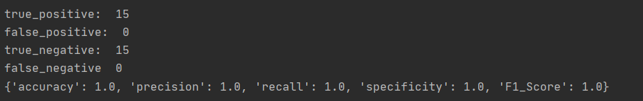
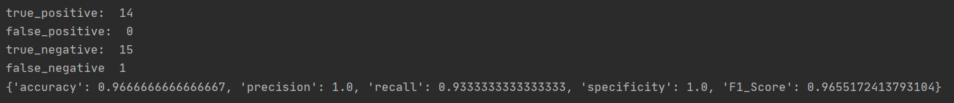
        print("true_positive: ", true_positive, "\nfalse_positive: ", false_positive,
              "\ntrue_negative: ", true_negative, "\nfalse_negative ", false_negative)
        accuracy = (true_positive + true_negative) / total_num  # 准确率（预测正确的样本与总样本数之比）
        precision = true_positive / (true_positive + false_positive)  # 精度（所有 预测 为阳性的样本中， 真值 为阳性的比例）
        recall = true_positive / (true_positive + false_negative)  # 召回率（所有 真值 为阳性的样本中， 预测 为阳性的比例）
        specificity = true_negative / (true_negative + false_positive)  # 特异性（所有 真值 为阴性的样本中， 预测 为阴性的比例）
        F1_Score = (2 * precision * recall) / (precision + recall)  # 精度与召回率的加权平均
        return {"accuracy": accuracy, "precision": precision, "recall": recall, "specificity": specificity,
                "F1_Score": F1_Score}

    # 获取某一类的样本中心点
    def get_center(self, key):
        if key in self.center_dict.keys():
            return self.center_dict[key]
        else:
            return []

    def get_center_dict(self):
        return self.center_dict

    # 获取所有类别的协方差矩阵
    def get_cov_dict(self):
        return self.sigma

# 将字典转换为列表（只保留每个键值对的值）
def dict_values_to_list(_dict_):
    if isinstance(_dict_, dict):
        return list(_dict_.values())
    else:
        return []


# feature表示样本特征，label表示对应的标签,m行n列共计m*n个子图
def visualization_2d(feature, label, m, n):
    plt.figure(figsize=(20, 20), dpi=80)
    img = [[] for i in range(m * n)]
    for i in range(m):
        for j in range(n):
            img[i * n + j] = plt.subplot(m, n, i * n + j + 1)
            plt.xlabel("x" + str(i))
            plt.ylabel("x" + str(j))
            # plt.xlim(-1, 9)
            # plt.ylim(-1, 9)
            # plt.legend()  # 显示图例
            plt.scatter(feature[:, i], feature[:, j], s=5, c=label, marker='.')
            plt.colorbar()  # 显示颜色条
            plt.grid(True)  # 显示网格线
    plt.show()


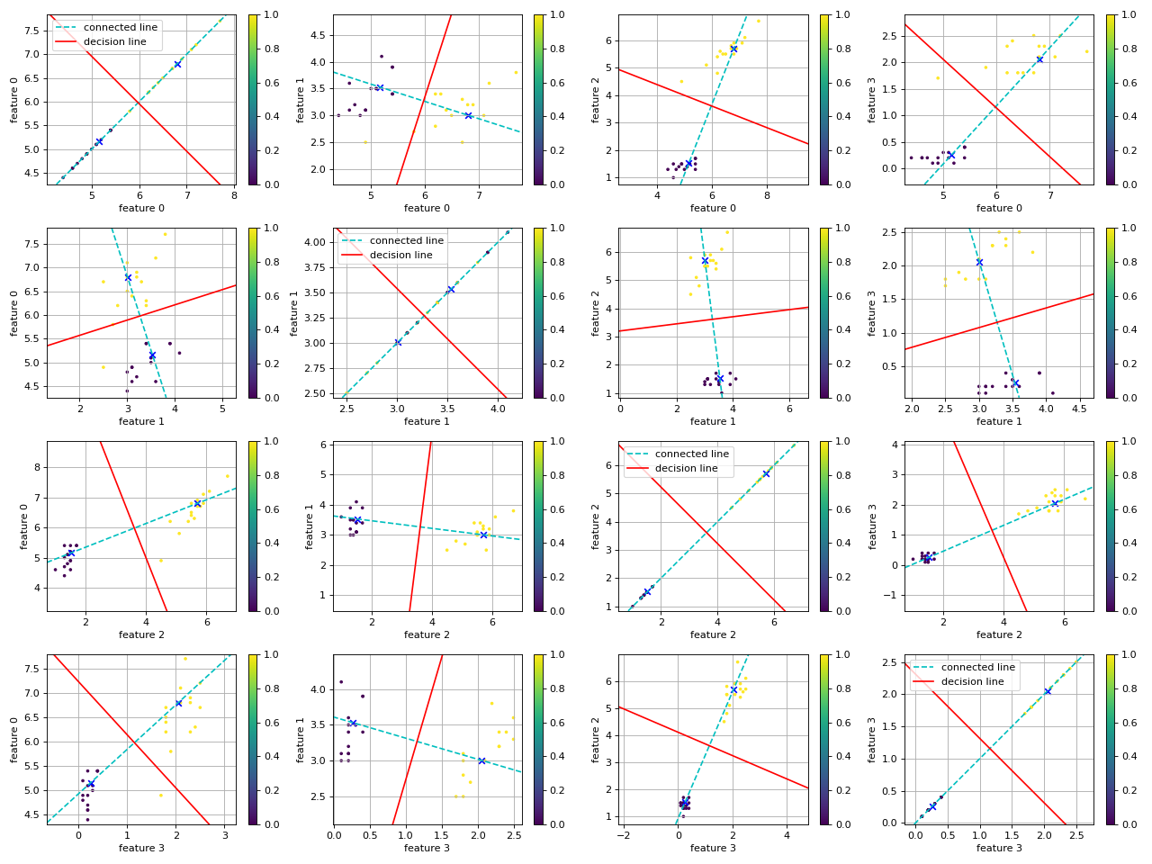
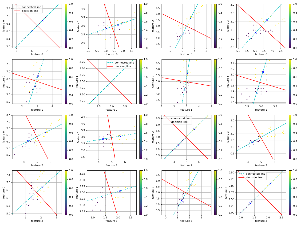
# 展示二维平面上，二分类问题的决策线（class_1和class_2）
# feature是样本特征集合，label是对应的标签集合，对每一维特征进行两两比较，n表示特征维数
def show_decision_line(feature, label, micd_classifier, class_1=0, class_2=0, n=0):
    plt.figure(figsize=(16, 12), dpi=80)  # 整张画布大小与分辨率
    img = [[] for i in range(n * n)]
    for i in range(n):
        for j in range(n):
            img[i * n + j] = plt.subplot(n, n, i * n + j + 1)
            center_1 = micd_classifier.get_center(class_1)
            center_2 = micd_classifier.get_center(class_2)
            c_1 = [center_1[i], center_1[j]]  # class_1类中心点的i, j两维的分量
            c_2 = [center_2[i], center_2[j]]  # class_2类中心点的i, j两维的分量
            center_3 = [(c_1[0] + c_2[0]) / 2, (c_1[1] + c_2[1]) / 2]  # 两点连线的中点
            k2, b2 = calculate_vertical_line(c_1, c_2)  # 两点中垂线的斜率和截距
            plt.scatter(feature[:, i], feature[:, j], c=label, s=20, marker='.')  # 整个样本集在特征0和2上的散点图
            plt.scatter(c_1[0], c_1[1], c='b', marker='x')  # 显示micd分类器计算的样本中心点
            plt.scatter(c_2[0], c_2[1], c='b', marker='x')
            plt.colorbar()  # 显示散点图的颜色条
            plt.grid(True)  # 显示网格线
            plt.axis('equal')  # 横纵坐标间隔大小相同
            plt.axline(c_1, c_2, color='c', linestyle="--", label="connected line")
            plt.axline(center_3, slope=k2, color='r', label="decision line")
            if i == j:
                plt.legend()  # 对角线上的子图显示出图例
            plt.xlabel("feature " + str(i))
            plt.ylabel("feature " + str(j))
            plt.tight_layout()  # 自动调整子图大小，减少相互遮挡的问题
    plt.show()


# 计算两点连线，返回斜率和纵截距（假设是二维平面上的点，并且用列表表示）
def calculate_connected_line(point_1, point_2):
    if len(point_1) != 2 or len(point_2) != 2:
        return None
    k = (point_1[1] - point_2[1]) / (point_1[0] - point_2[0])
    b = (point_1[0] * point_2[1] - point_2[0] * point_1[1]) / (point_1[0] - point_2[0])
    return k, b


# 计算两点中垂线，返回斜率和纵截距（假设是二维平面上的点，并且用列表表示）
def calculate_vertical_line(point_1, point_2):
    if len(point_1) != 2 or len(point_2) != 2:
        return None
    k = -(point_1[0] - point_2[0]) / (point_1[1] - point_2[1])
    b = (point_1[1] + point_2[1] + (point_1[0] + point_2[0]) * (point_1[0] - point_2[0]) / (
                point_1[1] - point_2[1])) / 2
    return k, b


# 去除某个类别的样本，返回两个numpy数组
def remove_from_sample(feature, label, _class_):
    new_feature = []
    new_label = []
    for index in range(len(label)):
        if label[index] != _class_:
            new_feature.append(feature[index])
            new_label.append(label[index])
    return np.asarray(new_feature), np.asarray(new_label)


if __name__ == '__main__':
    iris = datasets.load_iris()
    iris_x = iris.data
    iris_y = iris.target

    micd = MICDClassifier()  # 创建MICD分类器

    print(np.cov(micd.whitening(iris_x).T))  # 显示白化后的样本协方差矩阵

    # 显示白化前后的散点图
    # visualization_2d(iris_x, iris_y, 4, 4)
    # visualization_2d(np.asarray(iris_x_whitening).T, iris_y, 4, 4)

    # 去除线性可分的类（0类）
    iris_x_nonlinear, iris_y_nonlinear = remove_from_sample(iris_x, iris_y, 0)

    # 去除线性不可分类（1类）
    iris_x_linear, iris_y_linear = remove_from_sample(iris_x, iris_y, 1)

    # visualization_2d(iris_x_nonlinear, iris_y_nonlinear, 4, 4)  # 显示4个特征两两对比的散点图（包括自己比自己）

    # x_train, x_test, y_train, y_test = train_test_split(iris_x_linear, iris_y_linear, test_size=0.3)  # 使用线性可分的两类
    x_train, x_test, y_train, y_test = train_test_split(iris_x_nonlinear, iris_y_nonlinear, test_size=0.3)  # 使用线性不可分的两类

    micd.train(x_train, y_train)  # 训练

    print("========== center points of this two classes =========\n", micd.get_center_dict()
          , "\n======================================================")

    print("========== covariance matrix of this two classes =========\n", micd.get_cov_dict()
          , "\n======================================================")

    # print(np.asarray(dict_values_to_list(micd.predict(x_test))))  # 用numpy数组格式显示预测结果
    # print(y_test)
    performance = micd.performance(x_test, y_test, 1)  # 当以1类为阳性时，计算micd分类器的性能指标
    print(performance)

    # 展示每个特征两两对比图，显示决策线
    show_decision_line(x_test, y_test, micd, class_1=1, class_2=2, n=4)

• 在鸢尾花数据集上

  • 去除线性可分的类（1类），结果如下：
    
    

  • 去除线性不可分的类（0类），结果如下：