opencv-python图像处理4

一个很有趣的个人博客,不信你来撩 fangzengye.com

直方图

获取直方图

 cv.calcHist()

np.histogram()

例子

import numpy as np
import cv2 as cv
from matplotlib import pyplot as plt
img = cv.imread('home.jpg',0)
plt.hist(img.ravel(),256,[0,256]); plt.show()

对每个通道画图

import numpy as np
import cv2 as cv
from matplotlib import pyplot as plt
img = cv.imread('home.jpg')
color = ('b','g','r')
for i,col in enumerate(color):
    histr = cv.calcHist([img],[i],None,[256],[0,256])
    plt.plot(histr,color = col)
    plt.xlim([0,256])
plt.show()

应用遮挡框架

img = cv.imread('home.jpg',0)
# create a mask
mask = np.zeros(img.shape[:2], np.uint8)
mask[100:300, 100:400] = 255
masked_img = cv.bitwise_and(img,img,mask = mask)
# Calculate histogram with mask and without mask
# Check third argument for mask
hist_full = cv.calcHist([img],[0],None,[256],[0,256])
hist_mask = cv.calcHist([img],[0],mask,[256],[0,256])
plt.subplot(221), plt.imshow(img, 'gray')
plt.subplot(222), plt.imshow(mask,'gray')
plt.subplot(223), plt.imshow(masked_img, 'gray')
plt.subplot(224), plt.plot(hist_full), plt.plot(hist_mask)
plt.xlim([0,256])
plt.show()

将图像调整到曝光正常

import numpy as np
import cv2 as cv
from matplotlib import pyplot as plt
img = cv.imread('wiki.jpg',0)
hist,bins = np.histogram(img.flatten(),256,[0,256])
cdf = hist.cumsum()
cdf_normalized = cdf * float(hist.max()) / cdf.max()
plt.plot(cdf_normalized, color = 'b')
plt.hist(img.flatten(),256,[0,256], color = 'r')
plt.xlim([0,256])
plt.legend(('cdf','histogram'), loc = 'upper left')
plt.show()

cdf_m = np.ma.masked_equal(cdf,0)
cdf_m = (cdf_m - cdf_m.min())*255/(cdf_m.max()-cdf_m.min())
cdf = np.ma.filled(cdf_m,0).astype('uint8')
img2 = cdf[img]

关键代码

img = cv.imread('wiki.jpg',0)
equ = cv.equalizeHist(img)
res = np.hstack((img,equ)) #stacking images side-by-side
cv.imwrite('res.png',res)

自适应调整图像亮度

import numpy as np
import cv2 as cv
img = cv.imread('tsukuba_l.png',0)
# create a CLAHE object (Arguments are optional).
clahe = cv.createCLAHE(clipLimit=2.0, tileGridSize=(8,8))
cl1 = clahe.apply(img)
cv.imwrite('clahe_2.jpg',cl1)

2D直方图

2D Histogram in OpenCV

hist = cv.calcHist([hsv], [0, 1], None, [180, 256], [0, 180, 0, 256])

import numpy as np
import cv2 as cv
img = cv.imread('home.jpg')
hsv = cv.cvtColor(img,cv.COLOR_BGR2HSV)
hist = cv.calcHist([hsv], [0, 1], None, [180, 256], [0, 180, 0, 256])

2D Histogram in Numpy

hist, xbins, ybins = np.histogram2d(h.ravel(),s.ravel(),[180,256],[[0,180],[0,256]])

import numpy as np
import cv2 as cv
from matplotlib import pyplot as plt
img = cv.imread('home.jpg')
hsv = cv.cvtColor(img,cv.COLOR_BGR2HSV)
hist, xbins, ybins = np.histogram2d(h.ravel(),s.ravel(),[180,256],[[0,180],[0,256]])

Method - 2 : Using Matplotlib

hist = cv.calcHist( [hsv], [0, 1], None, [180, 256], [0, 180, 0, 256] )

import numpy as np
import cv2 as cv
from matplotlib import pyplot as plt
img = cv.imread('home.jpg')
hsv = cv.cvtColor(img,cv.COLOR_BGR2HSV)
hist = cv.calcHist( [hsv], [0, 1], None, [180, 256], [0, 180, 0, 256] )
plt.imshow(hist,interpolation = 'nearest')
plt.show()

https://docs.opencv.org/3.4/dd/d0d/tutorial_py_2d_histogram.html

直方图反投影

import numpy as np
import cv2 as cv
roi = cv.imread('rose_red.png')
hsv = cv.cvtColor(roi,cv.COLOR_BGR2HSV)
target = cv.imread('rose.png')
hsvt = cv.cvtColor(target,cv.COLOR_BGR2HSV)
# calculating object histogram
roihist = cv.calcHist([hsv],[0, 1], None, [180, 256], [0, 180, 0, 256] )
# normalize histogram and apply backprojection
cv.normalize(roihist,roihist,0,255,cv.NORM_MINMAX)
dst = cv.calcBackProject([hsvt],[0,1],roihist,[0,180,0,256],1)
# Now convolute with circular disc
disc = cv.getStructuringElement(cv.MORPH_ELLIPSE,(5,5))
cv.filter2D(dst,-1,disc,dst)
# threshold and binary AND
ret,thresh = cv.threshold(dst,50,255,0)
thresh = cv.merge((thresh,thresh,thresh))
res = cv.bitwise_and(target,thresh)
res = np.vstack((target,thresh,res))
cv.imwrite('res.jpg',res)

傅里叶变换

cv.dft()
cv.idft()

import numpy as np
import cv2 as cv
from matplotlib import pyplot as plt
img = cv.imread('messi5.jpg',0)
dft = cv.dft(np.float32(img),flags = cv.DFT_COMPLEX_OUTPUT)
dft_shift = np.fft.fftshift(dft)
magnitude_spectrum = 20*np.log(cv.magnitude(dft_shift[:,:,0],dft_shift[:,:,1]))
plt.subplot(121),plt.imshow(img, cmap = 'gray')
plt.title('Input Image'), plt.xticks([]), plt.yticks([])
plt.subplot(122),plt.imshow(magnitude_spectrum, cmap = 'gray')
plt.title('Magnitude Spectrum'), plt.xticks([]), plt.yticks([])
plt.show()

https://docs.opencv.org/3.4/de/dbc/tutorial_py_fourier_transform.html

模板匹配

在图像匹配出想要的对象

cv.matchTemplate()
cv.minMaxLoc()

例子

目标

import cv2 as cv
import numpy as np
from matplotlib import pyplot as plt
img = cv.imread('messi5.jpg',0)
img2 = img.copy()
template = cv.imread('template.jpg',0)
w, h = template.shape[::-1]
# All the 6 methods for comparison in a list
methods = ['cv.TM_CCOEFF', 'cv.TM_CCOEFF_NORMED', 'cv.TM_CCORR',
            'cv.TM_CCORR_NORMED', 'cv.TM_SQDIFF', 'cv.TM_SQDIFF_NORMED']
for meth in methods:
    img = img2.copy()
    method = eval(meth)
    # Apply template Matching
    res = cv.matchTemplate(img,template,method)
    min_val, max_val, min_loc, max_loc = cv.minMaxLoc(res)
    # If the method is TM_SQDIFF or TM_SQDIFF_NORMED, take minimum
    if method in [cv.TM_SQDIFF, cv.TM_SQDIFF_NORMED]:
        top_left = min_loc
    else:
        top_left = max_loc
    bottom_right = (top_left[0] + w, top_left[1] + h)
    cv.rectangle(img,top_left, bottom_right, 255, 2)
    plt.subplot(121),plt.imshow(res,cmap = 'gray')
    plt.title('Matching Result'), plt.xticks([]), plt.yticks([])
    plt.subplot(122),plt.imshow(img,cmap = 'gray')
    plt.title('Detected Point'), plt.xticks([]), plt.yticks([])
    plt.suptitle(meth)
    plt.show()

res = cv.matchTemplate(img,template,method)

mothod方法

methods = [‘cv.TM_CCOEFF’, ‘cv.TM_CCOEFF_NORMED’, ‘cv.TM_CCORR’,
‘cv.TM_CCORR_NORMED’, ‘cv.TM_SQDIFF’, ‘cv.TM_SQDIFF_NORMED’]

多目标侦测

import cv2 as cv
import numpy as np
from matplotlib import pyplot as plt
img_rgb = cv.imread('mario.png')
img_gray = cv.cvtColor(img_rgb, cv.COLOR_BGR2GRAY)
template = cv.imread('mario_coin.png',0)
w, h = template.shape[::-1]
res = cv.matchTemplate(img_gray,template,cv.TM_CCOEFF_NORMED)
threshold = 0.8
loc = np.where( res >= threshold)
for pt in zip(*loc[::-1]):
    cv.rectangle(img_rgb, pt, (pt[0] + w, pt[1] + h), (0,0,255), 2)
cv.imwrite('res.png',img_rgb)

https://docs.opencv.org/3.4/d4/dc6/tutorial_py_template_matching.html

节点线变换

cv.HoughLines(), cv.HoughLinesP()
lines = cv.HoughLines(edges,1,np.pi/180,200)

import cv2 as cv
import numpy as np
img = cv.imread(cv.samples.findFile('sudoku.png'))
gray = cv.cvtColor(img,cv.COLOR_BGR2GRAY)
edges = cv.Canny(gray,50,150,apertureSize = 3)
lines = cv.HoughLines(edges,1,np.pi/180,200)
for line in lines:
    rho,theta = line[0]
    a = np.cos(theta)
    b = np.sin(theta)
    x0 = a*rho
    y0 = b*rho
    x1 = int(x0 + 1000*(-b))
    y1 = int(y0 + 1000*(a))
    x2 = int(x0 - 1000*(-b))
    y2 = int(y0 - 1000*(a))
    cv.line(img,(x1,y1),(x2,y2),(0,0,255),2)
cv.imwrite('houghlines3.jpg',img)

概率节点变换

cv.HoughLinesP()

import cv2 as cv
import numpy as np
img = cv.imread(cv.samples.findFile('sudoku.png'))
gray = cv.cvtColor(img,cv.COLOR_BGR2GRAY)
edges = cv.Canny(gray,50,150,apertureSize = 3)
lines = cv.HoughLinesP(edges,1,np.pi/180,100,minLineLength=100,maxLineGap=10)
for line in lines:
    x1,y1,x2,y2 = line[0]
    cv.line(img,(x1,y1),(x2,y2),(0,255,0),2)
cv.imwrite('houghlines5.jpg',img)

https://docs.opencv.org/3.4/d6/d10/tutorial_py_houghlines.html

节点圈变换

cv.HoughCircles()

import numpy as np
import cv2 as cv
img = cv.imread('opencv-logo-white.png',0)
img = cv.medianBlur(img,5)
cimg = cv.cvtColor(img,cv.COLOR_GRAY2BGR)
circles = cv.HoughCircles(img,cv.HOUGH_GRADIENT,1,20,
                            param1=50,param2=30,minRadius=0,maxRadius=0)
circles = np.uint16(np.around(circles))
for i in circles[0,:]:
    # draw the outer circle
    cv.circle(cimg,(i[0],i[1]),i[2],(0,255,0),2)
    # draw the center of the circle
    cv.circle(cimg,(i[0],i[1]),2,(0,0,255),3)
cv.imshow('detected circles',cimg)
cv.waitKey(0)
cv.destroyAllWindows()

https://docs.opencv.org/3.4/da/d53/tutorial_py_houghcircles.html

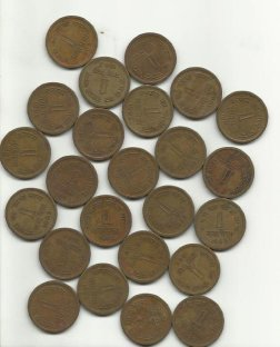
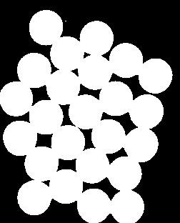
图像分割

cv.watershed()

import numpy as np
import cv2 as cv
from matplotlib import pyplot as plt
img = cv.imread('coins.png')
gray = cv.cvtColor(img,cv.COLOR_BGR2GRAY)
ret, thresh = cv.threshold(gray,0,255,cv.THRESH_BINARY_INV+cv.THRESH_OTSU)

https://docs.opencv.org/3.4/d3/db4/tutorial_py_watershed.html

前景提取使用抓取技术

cv.grabCut()

import numpy as np
import cv2 as cv
from matplotlib import pyplot as plt
img = cv.imread('messi5.jpg')
mask = np.zeros(img.shape[:2],np.uint8)
bgdModel = np.zeros((1,65),np.float64)
fgdModel = np.zeros((1,65),np.float64)
rect = (50,50,450,290)
cv.grabCut(img,mask,rect,bgdModel,fgdModel,5,cv.GC_INIT_WITH_RECT)
mask2 = np.where((mask==2)|(mask==0),0,1).astype('uint8')
img = img*mask2[:,:,np.newaxis]
plt.imshow(img),plt.colorbar(),plt.show()

使用遮挡罩进行改进

# newmask is the mask image I manually labelled
newmask = cv.imread('newmask.png',0)
# wherever it is marked white (sure foreground), change mask=1
# wherever it is marked black (sure background), change mask=0
mask[newmask == 0] = 0
mask[newmask == 255] = 1
mask, bgdModel, fgdModel = cv.grabCut(img,mask,None,bgdModel,fgdModel,5,cv.GC_INIT_WITH_MASK)
mask = np.where((mask==2)|(mask==0),0,1).astype('uint8')
img = img*mask[:,:,np.newaxis]
plt.imshow(img),plt.colorbar(),plt.show()

https://docs.opencv.org/3.4/d8/d83/tutorial_py_grabcut.html

All code source

https://docs.opencv.org/3.4/d2/d96/tutorial_py_table_of_contents_imgproc.html