Coursera-AndrewNg(吴恩达)机器学习笔记——第二周编程作业（线性回归）

一.准备工作

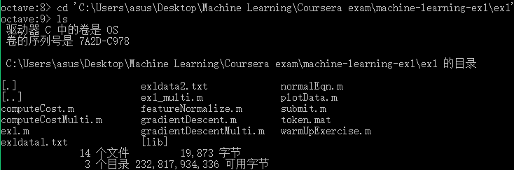
1. 从网站上将编程作业要求下载解压后，在Octave中使用cd命令将搜索目录移动到编程作业所在目录,然后使用ls命令检查是否移动正确。如：
   
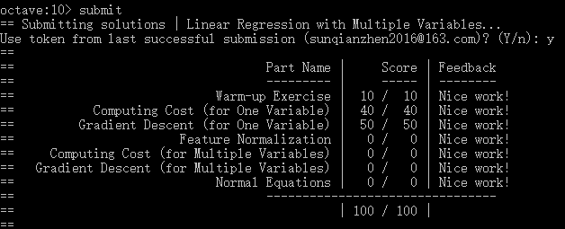
2. 提交作业：提交时候需要使用自己的登录邮箱和提交令牌，如下：
   
   

二.单变量线性回归

绘制图形：rx代表图形中标记的点为红色的x，数字10表示标记的大小。

plot(x, y, 'rx', 'MarkerSize', 10); % Plot the data

计算代价函数（Cost Funtion）：迭代次数1500，学习速率0.01. 　　iterations = 1500;　　alpha = 0.01;

注意需给原始数据X添加一列值为1的属性：X = [ones(m, 1), data(:,1)];　　theta = zeros(2, 1);

function J = computeCost(X, y, theta)　　%文件名为computeCost.m
m = length(y); % number of training examples
J = 1/(2*m)*sum((X*theta-y).^2);
end

梯度下降（Gradient Descent ）：

function [theta, J_history] = gradientDescent(X, y, theta, alpha, num_iters)　　%文件名为gradientDescent.m
m = length(y); % number of training examples
J_history = zeros(num_iters, 1);
for iter = 1:num_iters
    temp=X'*(X*theta-y);
    theta=theta-1/m*alpha*temp;
    J_history(iter) = computeCost(X, y, theta);
end
end

然后绘制出我们使用经过梯度下降求出的最优参数θ值所做预测的图形，如下：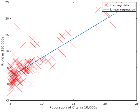

可视化J(θ):

使用表面图进行可视化：

theta0_vals = linspace(-10, 10, 100);　　%生成范围在[-10,10]之间100个点的线性行矢量，即维数为1*100的矩阵
theta1_vals = linspace(-1, 4, 100);　　%生成范围在[-1,4]之间100个点的线性行矢量，即维数为1*100的矩阵

J_vals = zeros(length(theta0_vals), length(theta1_vals));　　%对应的代价函数值，维数为100*100
% Fill out J_vals
for i = 1:length(theta0_vals)　　　　%计算代价函数值
    for j = 1:length(theta1_vals)
      t = [theta0_vals(i); theta1_vals(j)];
      J_vals(i,j) = computeCost(X, y, t);
    end
end

% Because of the way meshgrids work in the surf command, we need to transpose J_vals before calling surf, or else the axes will be flipped
J_vals = J_vals';　　　　%surface函数的特性，必须进行转置。其实就是因为θ0和θ1要和行列坐标x，y对齐。
% Surface plot
figure;
surf(theta0_vals, theta1_vals, J_vals)　　%绘制表面图
xlabel('\theta_0'); ylabel('\theta_1');

结果如下：从图中可看出代价函数值J(θ)有全局最优解（最低点）。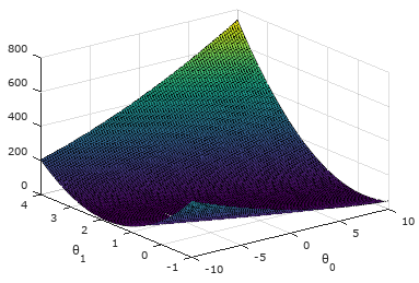

使用等高线图进行可视化：（logspace函数和linspace函数类似，此处作用生成将区间[10^-2,10³]等分20份的1*20矩阵）

figure;　　%这里的J_vals在前面进行了转置，所以此处不用转置！
contour(theta0_vals, theta1_vals, J_vals, logspace(-2, 3, 20))　　
xlabel('\theta_0'); ylabel('\theta_1');　　%用到了转义字符'\theta_0'和'\theta_1'.
hold on;
plot(theta(1), theta(2), 'rx', 'MarkerSize', 10, 'LineWidth', 2);

结果如下：可以看出我们求出的最优参数θ所对应的代价值，正好位于等高线图最低的位置！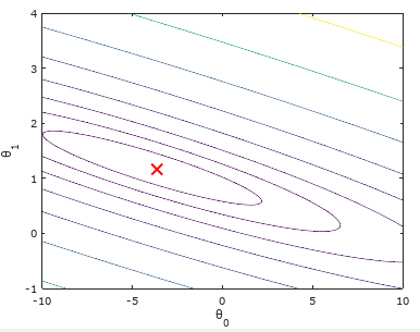

三.多变量线性回归（选做）

特征规则化：

function [X_norm, mu, sigma] = featureNormalize(X)　　%文件名为featureNormalize.m
X_norm = X;
mu = zeros(1, size(X, 2));　　%记录每个特征xi的平均值
sigma = zeros(1, size(X, 2));　　%记录每个特征xi的标准差值

for i=1:size(X,2),
  mu(i)=mean(X(:,i));　　　　%使用公式mean求平均值
  sigma(i)=std(X(:,i));　　　%使用公式std求标准差值
  X_norm(:,i)=(X_norm(:,i)-mu(i))/sigma(i);
end
end

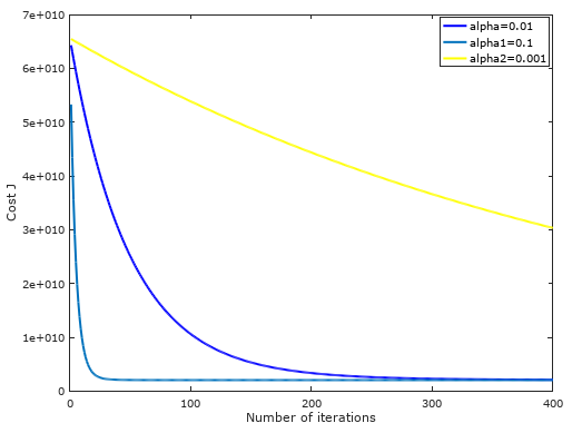
代价函数和梯度下降：和单变量相同（省略）

不同学习速率下，随着迭代次数的增加，代价函数值逐渐收敛图形：可以发现学习速率为0.01最为合适！

房价预测：Estimate the price of a 1650 sq-ft, 3 br house

% Estimate the price of a 1650 sq-ft, 3 br house
% ====================== YOUR CODE HERE ======================
% Recall that the first column of X is all-ones. Thus, it does
% not need to be normalized.
x_try=[1650 3];
x_try(1)=x_try(1)-mu(1);
x_try(2)=x_try(2)-mu(2);
x_try(1)=x_try(1)/sigma(1);
x_try(2)=x_try(2)/sigma(2);
price = [ones(1, 1) x_try]*theta; % 这里的theta是我们前面经过梯度下降求出的

 正规方程求参数theta:

function [theta] = normalEqn(X, y)
theta = zeros(size(X, 2), 1);
theta=pinv(X'*X)*X'*y;
end

无~