信用评分预测模型（四）--决策树算法

Author：Liedra
https://www.cnblogs.com/LieDra/

前言

下面将利用决策树算法对数据进行处理分析。

决策树介绍

决策树算法本质上是通过一系列规则对数据进行分类的过程。有监督学习。

常见的决策树算法有ID3，C4.5，CART。

• ID3：采取信息增益来作为纯度的度量。选取使得信息增益最大的特征进行分裂。
  信息熵是代表随机变量的复杂度（不确定度），条件熵代表在某一个条件下，随机变量的复杂度（不确定度）。
  而信息增益则是：信息熵-条件熵。
  因此在计算过程中先算限制的复杂度，再减去某种条件分裂下的复杂度，选择增益最大的那种条件。信息熵和条件熵可以通过各类样本占样本集合的比例来计算出。
  如果选择一个特征后，信息增益最大（信息不确定性减少的程度最大），那么我们就选取这个特征。
  但缺点是信息增益准则其实是对可取值数目较多的属性有所偏好，比如按照编号分类的话信息增益一定是很大的，只要知道编号，其它特征就没有用了，但是这样生成的决策树显然不具有泛化能力。
  为了解决这个问题，引入了信息增益率来选择最优划分属性。
• C4.5：用信息增益率来选择属性。
  信息增益率=信息增益/IV(a)
  这里的IV(a)衡量了以a属性划分时分成的类别数量，分成的类别数越大，IV(a)就越大。
  可以看出增益率准则其实对可取类别数目较少的特征有所偏好。
  因此实际上的C4.5算法不直接选择增益率最大的候选划分属性，而是在候选划分属性中找出信息增益高于平均水平的属性（保证特征效果较好），再从中选择增益率最高的（保证了不会出现如通过编号特征分类这种极端的情况）。
• CART：CART既能是分类树，又能是回归树。当CART是分类树时，采用GINI值作为分裂依据；当CART是回归树时，采用样本的最小方差作为分裂依据;
  分类树通过对象特征预测对象所属的类别，而回归树根据对象信息预测该对象的属性（并以数值表示）。

本文所采用的是CART分类树，分裂依据是GINI值。
由于时间限制，本文中的算法未考虑剪枝过程，后续将对此进行补充。

代码示例

'''
version:
author：liedra
Method:DecisionTree--可以直接使用原始数据，不用做处理，也可以选择处理后的数据。
'''
import pandas as pd
import numpy as np
import matplotlib.pyplot as plt
import numpy as np
# 导入决策树分类器

from sklearn import tree as treeee
from sklearn.tree import DecisionTreeClassifier   
# 导入训练集划分
from sklearn.model_selection import train_test_split 

# 开始读取文件，文件路径
readFileName="D:/study/5/code/python/python Data analysis and mining/class/dataset/german.xls"
# 读取excel
df=pd.read_excel(readFileName)
# x---前20列属性    一千行，二十列
x=df.ix[:,:-1] 
# y---第21列标签    一千行，一列
y=df.ix[:,-1]  
# 获得属性名
names=x.columns

# 获得train set 和 test set， random_state=0可删除，删除后每次运行程序结果不太一样，不删除的话为伪随机（每次运行程序结果相同）
# x_train,x_check,y_train,y_check=train_test_split(x,y,random_state=120) 

# 测试最优深度  测试完成后可以将此处注释掉
# 迭代50次
# '''
def train_test():
    index_of_best = {}
    for i0 in range(1,21):
        index_of_best[i0]=0
    for i1 in range(50):
        x_train,x_test,y_train,y_test=train_test_split(x,y,test_size=0.4,random_state=i1+1)
        x_test2,x_check,y_test2,y_check=train_test_split(x_test,y_test,train_size=0.25,random_state=i1+2)
        # x_train,x_check,y_train,y_check=train_test_split(x,y,random_state=i1+1)

        list_average_accuracy=[]
        depth=range(1,21)
        # 对不同深度进行测试
        for i in depth:
            # max_depth=4
            # 限制决策树深度可以降低算法复杂度，获取更精确值
            tree = DecisionTreeClassifier(max_depth=i,random_state=38) #可删除后面的random_state以实现随机
            # 开始训练
            tree.fit(x_train,y_train)
            # 训练集score 
            accuracy_training=tree.score(x_train,y_train)
            # 测试集score
            accuracy_test=tree.score(x_check,y_check)
            # 平均score
            # average_accuracy=(accuracy_training+accuracy_test)/2.0
            print("depth %d accuracy on the check subset:" % (i),accuracy_training,'   ',accuracy_test)
            list_average_accuracy.append(accuracy_test)

        # 获得score最大的对应score值
        max_value=max(list_average_accuracy)
        # 获得score最大深度对应的索引，索引是0开头，结果要加1，即深度best_depth
        best_depth=list_average_accuracy.index(max_value)+1
        print("best_depth:",best_depth)
        # 这里得到的是random=47时,
        index_of_best[best_depth]+=1
    print(index_of_best)

train_test()
# '''


# 把之前对应的for循环中的最优深度单独拿出来构造最优的树，并且输出
x_train,x_test,y_train,y_test=train_test_split(x,y,test_size=0.4,random_state=47)
x_test2,x_check,y_test2,y_check=train_test_split(x_test,y_test,train_size=0.25,random_state=48)
best_tree = DecisionTreeClassifier(max_depth=4,random_state=38)
best_tree = best_tree.fit(x_train,y_train)
accuracy_training=best_tree.score(x_train,y_train)
accuracy_test=best_tree.score(x_test,y_test)
print("decision tree:") 
print("accuracy on the training subset:{:.3f}".format(best_tree.score(x_train,y_train)))
print("accuracy on the test subset:{:.3f}".format(best_tree.score(x_check,y_check)))
print(best_tree.predict(x_check))

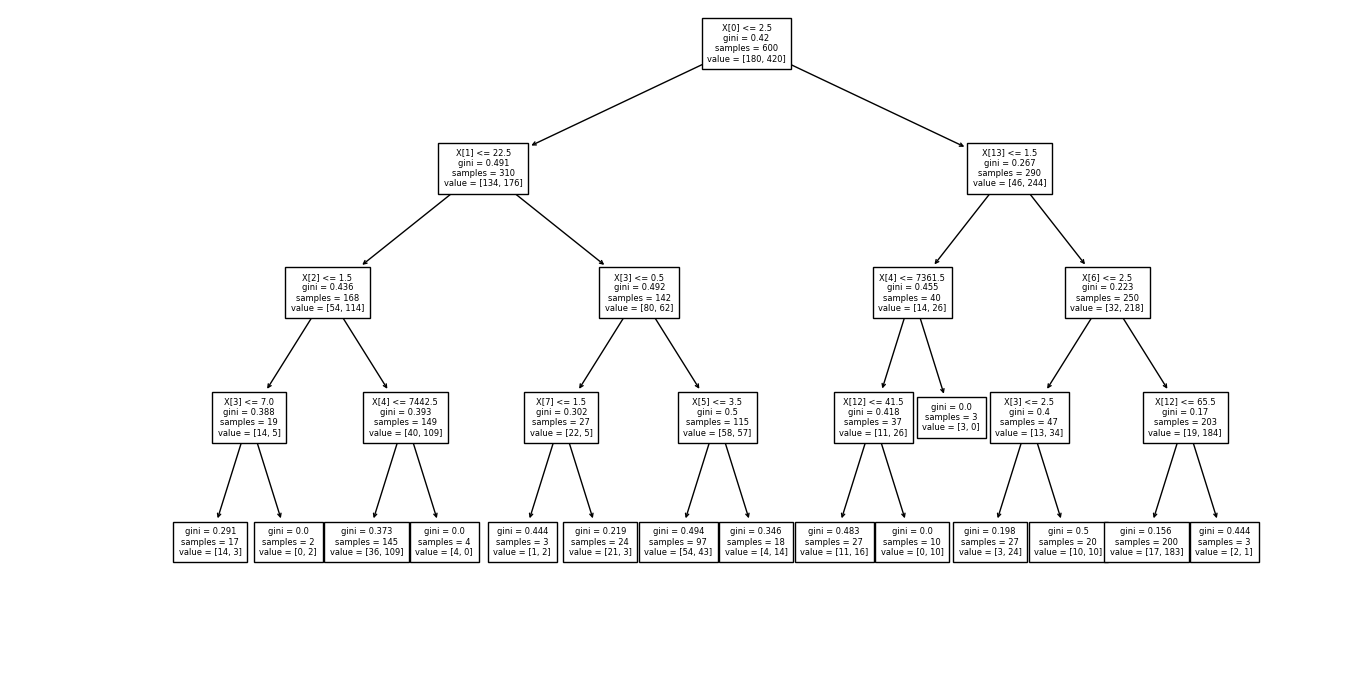
# 作图
plt.figure(figsize=(14,8))
treeee.plot_tree(best_tree,fontsize=6)   
# 这里可能会出现报错module 'sklearn.tree' has no attribute 'plot_tree'，
# 原因是版本较低，要0.21以上才有，而一般的可能只是0.19版本
# 更新方式可以参考网上资料，此处不再赘述
plt.show()

得到效果图如下：

当修改最大深度为9时（即max_depth=9），得到的效果图如下：

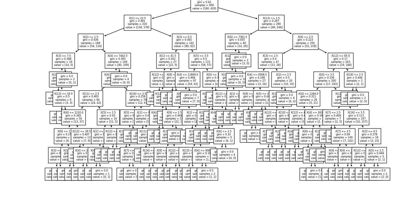
树越深，它就分裂的越多，更能捕获有关数据的信息。
但是与此同时需要的计算时间可能也会增加，而且有可能出现过拟合的情况。
我们在深度1-20之间分别进行测试，通过分析模型的score，最后选择了最大深度为4的情况。
在此深度下，已经能够对我们的测试数据有较好的拟合。