
Python 机器学习及实践 Coding 无监督学习经典模型 数据聚类 and 特征降维
无监督学习(部分代码有错误更改中)
着重于发现数据本身的分布特点 (不需要对数据进行标记)节省大量人力 数据规模不可限量
1 发现数据群落 数据聚类 也可以寻找 离群样本
2 特征降维 保留数据具有区分性的低维特征
这些都是在海量数据处理中非常实用的技术
数据聚类
K均值算法(预设聚类的个数 不断更新聚类中心 迭代 ,是所有数据点到其所属聚类中心距离平方和趋于稳定)
过程
①首先 随机布设K个特证空间内的点作为初始的聚类中心
②然后 对于根据每个数据的特长向量 从K个聚类中心中 寻找距离最近的一个 并且把该数据标记为从属与这个聚类中心
③接着 在所有数据都被标记了聚类中心之后 根据这些数据新分配的类簇 重新对K个聚类中心做计算
④如果一轮下来 所有数据从属的聚类中心与上一次的分配的类簇没有变化 那么迭代可以 停止 否则回到②继续循环
K-mans算法在手写体数字图像数据上的使用示例
import numpy as np
import matplotlib.pyplot as plt
import pandas as pd

from sklearn.cluster import KMeans

#使用panda 读取训练数据集 和 测试数据集
digits_train = pd.read_csv('https://archive.ics.uci.edu/ml/machine-learning-databases/optdigits/optdigits.tra',header=None)
digits_test=pd.read_csv('https://archive.ics.uci.edu/ml/machine-learning-databases/optdigits/optdigits.tes',header=None)

#从训练数据集与测试数据集上都分离出64维度的像素特征与1维度的数字目标
x_train=digits_train[np.arange(64)]#np.arange
y_train=digits_train[64]

x_test=digits_test[np.arange(64)]
y_test=digits_test[64]

#初始化Kmeans 模型 并设置聚类中心数量为10
kmeans=KMeans(n_clusters=10)
kmeans.fit(x_train,y_train)
y_predict=kmeans.predict(x_test)

#使用ARI 进行K-means 聚类性能评估
from sklearn import metrics
print(metrics.adjusted_rand_score(y_test,y_predict))
性能测评:
①被用来评估的数据本身带有正确的类别信息 使用ARI ARI指标与分类问题中计算准确性的方法类似,同时也兼顾到了类簇无法和分类标记一一对应的问题
②如果被用于评估的数据没有所属类别,那么我们习惯使用轮廓系数来度量聚类结果的质量。轮廓系数同时兼顾了聚类的凝聚度和分离度
用于评估聚类的效果并取值范围为[-1,1]。轮廓系数值越大,表示聚类效果越好。
具体计算步骤如下(暂略)
利用轮廓系数评价不同类簇数量的K-maens聚类实例(改错中)
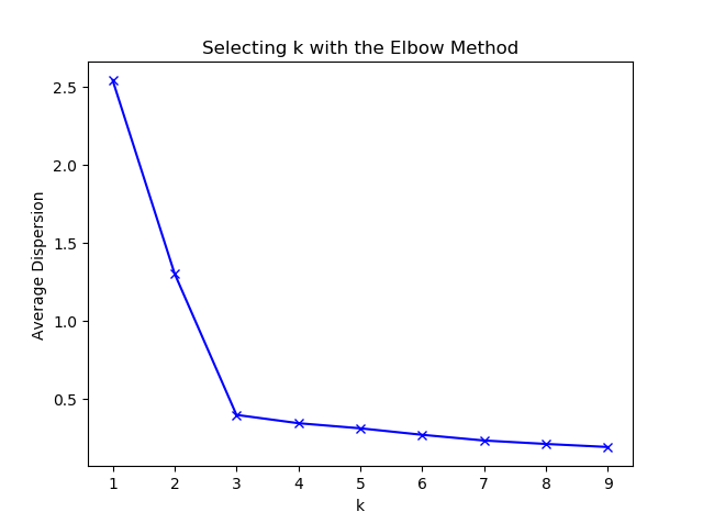
“ 肘部 ” 观察法示例
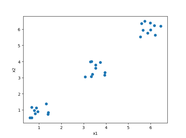
import numpy as np
from sklearn.cluster import KMeans
from scipy.spatial.distance import cdist

import matplotlib.pyplot as  plt

#使用均匀分布函数随机三个簇,每个簇周围有10个样本
cluster1=np.random.uniform(0.5,1.5,(2,10))
cluster2=np.random.uniform(5.5,6.5,(2,10))
cluster3=np.random.uniform(3.0,4.0,(2,10))

#绘制30个数据样本的分布图像
x=np.hstack((cluster1,cluster2,cluster3)).T
plt.scatter(x[:,0],x[:,1])
plt.xlabel('x1')
plt.ylabel('x2')
plt.show()

#测试9种不同聚类中心数量下 每种情况的聚类质量 并作图
K=range(1,10)
meandistotrtions=[]

for k in K:
    kmeans=KMeans(n_clusters=k)
    kmeans.fit(x)
    meandistotrtions.append(sum(np.min(cdist(x,kmeans.cluster_centers_,'euclidean'),axis=1))/x.shape[0])

plt.plot(K,meandistotrtions,'bx-')
plt.xlabel('k')
plt.ylabel('Average Dispersion')
plt.title('Selecting k with the Elbow Method')
plt.show()
输出图片:
特征降维
1实际项目中遭遇特征维度非常之高的训练样本,而往往又无法凭借自己的领域知识人工构建有效特征
2肉眼只能观测三个维度的特征 降低数据维度 同时也维数据展现提供了可能
主成分分析(PCA分析)
线性相关矩阵秩的计算样例
import numpy as np
M=np.array([[1,2],[2,4]])
np.linalg.matrix_rank(M,tol=None)
如果使用PCA分析的话 这个矩阵的 秩 是1 也就是说 在多样性程度上这个矩阵只有一个自由度
我们可以把PCA当作特征选择,只是和普通理解的不同,这种特征选择是首先把原来的特征空间做了映射,使得新的映射后特征空间的数据彼此正交。
这样一来,我们通过主成分分析就尽可能保留下具有区分性的低纬数据特征。
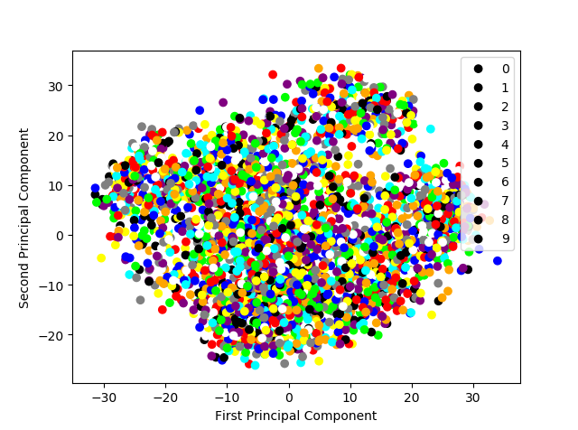
显示手写体数字图片经PCA压缩后的二维空间分布
import pandas as pd
import numpy as np

#导入PCA
from sklearn.decomposition import PCA
from matplotlib import pyplot as plt

#使用panda 读取训练数据集 和 测试数据集
digits_train = pd.read_csv('https://archive.ics.uci.edu/ml/machine-learning-databases/optdigits/optdigits.tra',header=None)
digits_test=pd.read_csv('https://archive.ics.uci.edu/ml/machine-learning-databases/optdigits/optdigits.tes',header=None)

#从训练数据集与测试数据集上都分离出64维度的像素特征与1维度的数字目标
x_digits=digits_train[np.arange(64)]#np.arange
y_digits=digits_train[64]

#初始化一个可以将到尾都特征向量(六十四维)压缩值二个维度的PCA
estimator=PCA(n_components=2)
x_pca=estimator.fit_transform(x_digits)

#显示10类手写体数字图片经过PCA压缩后的2 维空间分布
def plot_scatter():
    colors=['black','blue','purple','yellow','white','red','lime','cyan','orange','gray']

    for i in range(len(colors)):
        px = x_pca[:,0][y_digits.as_matrix() ==i]
        py = x_pca[:, 1][y_digits.as_matrix() == i]
        plt.scatter(px,py,c=colors)

    plt.legend(np.arange(0,10).astype(str))
    plt.xlabel('First Principal Component')
    plt.ylabel('Second Principal Component')
    plt.show()

plot_scatter()
输出图片:
使用原始像素特征和经PCA压缩重建的低维特征,在相同配置的支持向量机(分类)模型上分别进行图像识别
import pandas as pd
import numpy as np
from sklearn.svm import LinearSVC#基于线性核函数的支持向量机分类器
#导入PCA
from sklearn.decomposition import PCA
from sklearn.metrics import classification_report

#使用panda 读取训练数据集 和 测试数据集
digits_train = pd.read_csv('https://archive.ics.uci.edu/ml/machine-learning-databases/optdigits/optdigits.tra',header=None)
digits_test=pd.read_csv('https://archive.ics.uci.edu/ml/machine-learning-databases/optdigits/optdigits.tes',header=None)

#从训练数据集与测试数据集上都分离出64维度的像素特征与1维度的数字目标
x_train=digits_train[np.arange(64)]#np.arange
y_train=digits_train[64]

x_test=digits_test[np.arange(64)]#np.arange
y_test=digits_test[64]

#使用默认配置初始化LinearSVC 对原始六十四维像素特征的训练数据进行建模,并在测试数据上做出预测 存储在y_predict中
svc=LinearSVC()
svc.fit(x_train,y_train)
y_predict=svc.predict(x_test)

#使用PCA 将数据压缩到20个维度
estimator=PCA(n_components=20)

#利用训练特征决定(fit)20个正交维度的方向,并转化(transform)原训练特征
pca_x_train=estimator.fit_transform(x_train)
#测试特征也按照上述的20个正交维度方向进行转化
pca_x_test=estimator.transform(x_test)

#使用默认配置初始化LinearSVC 对压缩后的二十维特征的训练数据进行建模 并在测试数据上做出预测 存储在pca_y_predict 中
pca_svc=LinearSVC()
pca_svc.fit(pca_x_train,y_train)
pca_y_predict=pca_svc.predict(pca_x_test)

print(svc.score(x_test,y_test))
print(classification_report(y_test, y_predict,target_names=np.arange(10).astype(str)))

print(pca_svc.score(pca_x_test,y_test))
print(classification_report(y_test, pca_y_predict,target_names=np.arange(10).astype(str)))

 浙公网安备 33010602011771号