【论文阅读】Chinese Relation Extraction Using Lattice GRU[ITNEC2020]

论文地址：https://ieeexplore.ieee.org/abstract/document/9085019

Abstract

现有的中文实体关系抽取模型大多采用基于字符或单词输入的方法。然而，基于词的输入法忽略了句子中潜在的词信息，并且会受到分词错误传播的影响。为了解决这个问题，我们引入了一个格模型lattice model，它可以合并输入的单词和字符，并使用BiGRU代替BiLSTM。经过对比实验，我们的模型取得了较好的效果。

I.  INTRODUCTION

RE是信息抽取领域的一个重要研究课题[1]。RE的主要目的是标记非结构化文本中两个特定实体对之间的语义关系，即在命名实体识别的基础上，找到非结构化文本中的实体关系，形成结构化数据进行存储和检索。该技术还可以用于其他许多自然文本处理任务，如知识图构建、问答系统构建等[2]。

传统的关系分类方法大多是基于模式匹配或使用附加的nlp语义特征。其中，模式匹配已经取得了较好的性能，表现为Rink利用大量语料库提取的特征来训练SVM分类[3]。这些方法的缺点是需要更多的人力和计算成本，并且会导致额外的传播误差。更糟糕的是，随着训练数据的变化，模型的泛化能力不强，性能不够稳定。

近年来，深度学习在特征提取任务中显示出前所未有的优势[4]。根据输入粒度的不同，将主流的中文关系抽取方法分为两类。一种是基于字符输入，另一种是基于单词输入，基于单词输入的模型会出现切分错误。

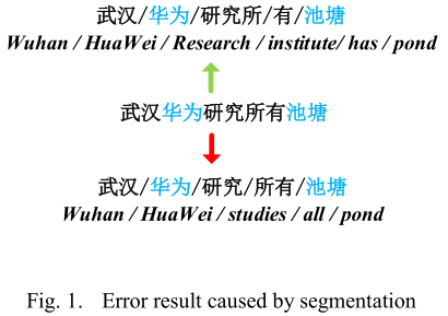
例如，如图1所示，汉语句子“武汉华为研究所有池塘”，这句话中有两个实体“华为”和“池塘”。如果分词正确，应该是“武汉/华为/研究/所有/池塘”。此时，“华为”与“池塘”的关系应该是一个整体。但如果将句子错误地分割为“武汉/华为/研究/所有/池塘”，则“华为”与“池塘”的关系将成为研究对象。也就是说，随着分词结果的变化，实体对之间的关系可能会变得完全不同。因此，无论是基于字符输入的模型还是基于单词输入的模型都不能很好地利用句子中潜在的语义信息。当模型的训练数据较小时，这种情况会变得更加严重。为了解决这个问题，张等提出了一种格LSTM结构来表示句子中的单词[5]。

本文引入格型LSTM的思想，改进了基于BiLSTM注意网络和字符输入的实体关系抽取模型。由于LSTM结构复杂，训练时间长，我们将网络层改为GRU单元。

我们在三个中文数据集上进行了一组实验，并与现有的一些模型进行了比较，结果表明我们的模型比其他模型有更好的改进。

II.  RELATED WORK 

近年来，人们提出了各种各样的方法来进行再学习，深度学习就是其中之一。2015年，Zhang和Wang提出了一种基于双向RNN模型的关系抽取方法。由于梯度消失的问题，RNN可以处理的文本长度是有限的。因此，带有注意机制的LSTM逐渐被应用到实体关系抽取的任务中[6]。

针对汉英语言的差异，提出了基于字符和基于单词的模式[7]。但是，这些方法都没有注意到输入粒度的问题，Zhang等人提出了一种基于lattice LSTM的模型，在基于单词粒度输入的模型中增加了一个额外的单词LSTM单元，使得网络能够利用词汇信息。

最后，我们的工作是在实体抽取模型上修改模型的输入层和特征层，并用GRU代替LSTM以缩短训练时间。

III. MODEL 

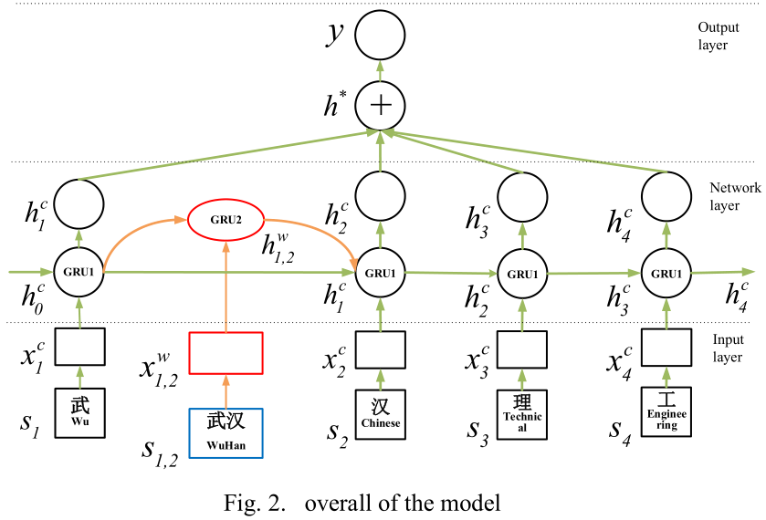
在本节中，我们将详细解释注意格GRU模型。如图2所示，该模型的整体结构分为3个部分：

· 输入表示层：给定一个特定的汉语句子和一个目标实体对，每个字符和单词将被转换成向量并输入到模型中。

· Lattice-GRU网络层：在前面的步骤之后，我们得到输入嵌入，然后将这些嵌入放到网络中来调整网络参数。

· 关系分类输出层：

1）注意层：对网络层的结果进行加权。

2）输出层：利用softmax分类器对注意层输出的场景级特征向量进行分类和预测。

我们将在后面的章节中详细解释这些章节。

A. Input presentation layer 

Given a Chinese sentence $S=\{s_1,s_2,s_3,...,s_N\}$ consisting of $N$ characters, and the identified entity pairs $e_1$,$e_2$. In order to integrate character and word information in the model input, we need to embed characters and words at the same time.

1) char input embeddings  

如图2所示，首先我们仍然使用句子中的字符作为主要道路main road上GRU单元格的输入（绿色部分），这里我们使用Word2Vec[8]中的Skip Gram模型, For each character $s_i$ , finding the existing character embedding matrix $x_i^{v}\in \cal{R^{d_c^{|V|}}}$, where $V$ represents the size of the character embedding matrix, and $d_c$ refers to the dimension of the character embedding matrix.

Each input character has a corresponding position $pf$ for the two entities in the sentence. We convert the position information into a vector and merge it with word embeddings. As is shown in Figure 3, there is a sentence $S={s_1,s_2,s_3,...,s_M}$ consisting of $M$ characters, and there is an entity $e={s_b,...,s_e}$ in it, here the subscript of $s$ represents the position of this character in the sentence. Here the relative position of $s_u$ to entity $e$ is $u-b$ , and the relative position of $s_v$ to entity $e$ is $v-e$. If the character in the entity $e$, its relative position to entity $e$ is specified as zero.

For each character input in the sentence, we calculated its relative to the two entities $e_1$ and $e_2$ as $pf_1$ and $pf_2$. By querying the position embedding table $x_i^{pf}\in \cal{R^{d_p^{|VP|}}}$, we can transform $pf_1$ and $pf_2$ into two position vectors $x_i^{pf_1}$ and  $x_i^{pf_2}$. Here the $d_p$ represents the dimension of the position embedding matrix, and $VP$ represents the size of the position embedding matrix. Then merge three embeddings together to get the result.

$x_i^c\left[\begin{matrix} x_i^V\\x_i^{pf_1}\\x_i^{pf_2}\end{matrix}\right]\tag{2}$

Finally, the obtained $x_i^c$ is the character vector input to the GRU unit on the main road.

2) word input embeddings 

从前面的描述可以看出，格模型不仅有基本的字符输入，而且需要句子中潜在的单词作为输入，以增加模型能够捕捉到的信息。因此，我们需要获得句子中的单词，然后将它们处理成与字符输入向量具有相同维数的向量，然后将它们组合到额外的单词格单元中。

In order to match the words in the sentence, we collected a large amount of raw text and segment it to build a word dictionary $\cal{D_w}$. Let $s_{b,e}$ be a word consisting of the $b$-th character to the $e$-th character in the sentence, here using Word2Vec to represent the word as a real-valued ${x_s^W}_{b,e} \in \cal{R}^{d_w|VW|}$, Here $d_w$ is the dimension of the word embedding vector, and $VW$ is the final dictionary size.

B. Network layer  

1)  Basic GRU Model 

通常，标准LSTM模型是RNN的一种特殊类型[9]。该模型的核心思想是“细胞状态”。这种结构类似于传送带，信息可以流向下游单元而不会丢失。此外，LSTM还能够通过一个设计良好的结构“gate”删除或添加单元状态信息。门可以选择要通过LSTM单元的信息。对于每个LSTM单元，有四个门：输入门、输出门、忘记门和更新门。

经典的GRU模型是LSTM的一个变体[10]。GRU将遗忘门和输入门合并为一个更新门，该门将单元状态和隐藏状态混合在一起。与LSTM相比，GRU的结构更简单，在训练数据集很大的情况下可以节省大量的时间。隐层状态的计算公式如下：

$z_i=\sigma(W_z\cdot [h_{i-1},x_i])$

$r_i=\sigma(W_r\cdot [h_{i-1},x_i])$

$\tilde{h}_i=tanh(W_{\tilde{h}}\cdot [r_i*h_{i-1},x_i])$

$h_i=(1-z_i)*h_{i-1}+z_i*\tilde{h}_i$

Here, $\sigma$ refers to the sigmoid function. $\tilde{h}_i$ is the output candidate dataset before data screening. It can be seen from the formula that the ordinary GRU network can only carry the character information in the sentence between the cell to cell.。$\tilde{h}_i$ 是数据筛选前的输出候选数据集。从公式中可以看出，普通的GRU网络只能在单元间传递句子中的字符信息。

2)  Lattice GRU Model 

通过上一节的介绍，我们可以知道一个简单的GRU模型不能充分利用句子中有用的单词信息，为了提高模型获取句子底层信息的能力，我们需要在单词输入的基础上增加GRU单元。

首先，给我一个词$s_{b,e}$在句子中，$b$和$e$表示句子中单词的开头和结尾。然后，将这个单词与我们构建的单词词典进行匹配，得到这个单词的单词嵌入表示：

$x_{b,e}^w = e^w(s_{b,e})$

$e^w$这里表示与单词字典匹配的操作。here represents the operation that matches the word dictionary.

The hidden state of the GRU2 unit output is represented by $h_{b,e}^w$, and its calculation formula is as follows:

$z_{b,e}^w=\sigma(W_z\cdot [h_b,x_{b,e}^w])$

$r_{b,e}^w=\sigma(W_r\cdot [h_b,x_{b,e}^w])$

$\tilde{h}_{b,e}^w=tanh(W\cdot [{r_{b,e}^w}*h_b,x_{b,e}^w])$

$h_{b,e}^w=(1-z_{b,e}^w)*h_b+{z_{b,e}^w}*{\tilde{h}_{b,e}^w}$

Among the formulas, $z_{b,e}^w$ and $r_{b,e}^w$ are the update gate and reset gate of word level input. As is shown in Figure 2, the hidden state $h_b^c$ at the beginning of the word combines the hidden state $h_{b,e}^w$ of the at the end of the word, and then enter into the GRU1 cell at the end of the word. Since the importance of each word is different, an additional gate is needed here to calculate the influence proportion of each word:

$z_{b,e}^c=\sigma(W_z^w\cdot [h_{b,e}^w,x_e^c])$

Because the degree of influence are different among the hidden state inputs to the $h_e^c$, normalized processing is used here to calculate the importance of each input. The hidden state for the $j$th character is calculated as follows:

$h_j^c=\sum_{b\in \{b^{'}|s_{b^{'}j}\in \cal{D}\}}\alpha_{b,j}^c\bigodot h_{b,j}^w+\alpha_j^c\bigodot \tilde{h}_j^c$

Here the $\alpha_{b,e}^c$ and $\alpha_{e}^c$ are normalization factors for calculating用于计算的归一化因子 $h_e^c$, the sum of them is 1, it represent the input proportion of each word and characters.

$\alpha_{b,j}^c=\frac{exp(z_{b,j}^c)}{exp(z_j^c)+\sum_{b^{'}\in \{b^{''}|s_{b^{''}e}\in \cal{D}\}}exp(z_{b^{'},j}^c)}$

$\alpha_{j}^c=\frac{exp(z_{j}^c)}{exp(z_j^c)+\sum_{b^{'}\in \{b^{''}|s_{b^{''}e}\in \cal{D}\}}exp(z_{b^{'},j}^c)}$

 这种结构使得模型能够动态地关注句子中的单词信息。在反向传播过程中，模型会调整超参数以获得更好的性能。

C. Relationship classification output layer 

1)  Attention layer 

近年来，注意机制在机器翻译和语音识别等许多任务中表现出了良好的性能。标准的注意机制已用于各种自然语言处理问题。

在这里，我们使用标准注意机制来解决关系分类问题。在上一节中，我们可以知道如何获得模型的隐藏状态输出序列${ℎ_1,ℎ_2,ℎ_3…ℎ_M}$ , $H=[ℎ_1,ℎ_2,ℎ_3…ℎ_M]$, 其中$M$是指句子的字符长度。我们使用字符级注意机制character-level来进行合并$h_i$ 到句子级特征向量中，$r$是这些隐藏层的输出向量的加权和。具体计算公式如下：

$M=tanh(H)$

$\alpha = softmax(w^TM)$

$r = H\alpha^T$

Here $w$ is the training parameter and $\alpha$ is the weight vector of the hidden state $H$. Here $H\in \cal{R}^{d_c}$, $d_c$ is the dimension of each character output from the hidden layer. Then, we can get the final output of the attention layer by the following formula:

$h^{*} = tanh(r)$

2)  Relation Classifier

经过字符级的注意处理，得到句子级的加权向量。然后，利用softmax多分类器对注意层的输出进行评价。实际上，softmax输出是训练集中每个关系的概率，关系概率之和为1。softmax多分类器表示如下：

$S_{in} = W_sh^{*}+b_s$

$\hat{p}(y|S)=softmax(S_{in})$

Here $y$ is the estimated probability for each realation, and then the result with the highest score is appointed as the last predicted relation label:

$\hat{y}=argmax\hat{p}(y|S)$

$\theta$ 表示模型中所有超参数的集合。每次计算损失函数时，模型都会调整参数。

在训练过程中，为了防止所有隐单元的协同适应cooperative adaptation，在每一训练批的前向传播中都以一定的概率保留了一些神经元。这使得网络更简单，并防止模型过度拟合[11]。

IV.  EXPERIMENTS 

A. Experiment settings

1) Dataset

我们在两个不同的数据集上进行实验来评估模型。由于该模型主要针对中文实体关系的提取，因此所使用的数据集是完整的公共中文RE数据集。其中一个数据集是中文文献NER-RE数据集Ch-L[12]，它是github上的一个开源数据集。该数据集对730篇中文文献进行处理，构建了一个包含7个实体标签和9个关系标签的中文NER-RE数据集。另一个是在其他中文实体关系抽取模型中发现的公共数据集ChRE，该数据集还定义了9个实体关系。

2) Hyper-parameter settings

在验证数据集上通过网格搜索grid search调整实验超参数。结果表明，字符嵌入和单词嵌入的最佳维数为50，最佳隐单元数为200，字符嵌入和单词嵌入的脱落值为0.5。通过训练过程中的调整和验证，将模型的初始学习率lr设置为0.015，每次迭代的衰减率设置为0.05。对于其他一些参数，由于对整个模型影响不大，我们借鉴其他模型的经验来设置初始化参数。The experimental hyperparameters are adjusted by grid search on the validated dataset. Finally, it has been found that the optimal dimension for character embedding and word embedding is 50, the optimal number of hidden units is 200, and the Dropout value of character embedding and word embedding is set to 0.5. Through the adjustment and verification during the training, the initial learning rate lr of the model is set to 0.015, and the attenuation rate of each iteration is set to 0.05. For some other parameters, since it has little effect on the overall model, we learn from the experience of other models to set the initialization parameters.

B. Experiment results 

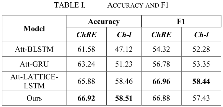
表1比较了我们的模型与其他关系分类方法的精度和F1。

BILSTM: Zhang et al. use some external NLP toolkits and bidirectional LSTM networks to learn sentence-level features.

Att-BLSTM: Zhou et al. add the sentence-level attention mechanism to the BILSTM model, making the model simpler without the help of external nlp toolkit and vocabulary resources.

Att-GRU: This method is a variant implementation of Att-BLSTM. The basic principle is roughly the same. The model's training time is shorter while maintaining the performance of the model.

Att-LATTICE-LSTM: Zhang et al., introduce a lattice structure into then Att-BLSTM model, so that the model can obtain word information in sentences, and they applied this model to the task of entity extraction. Here we compare it as a baseline model.

Att-LATTICE-LSTM:Zhang等人在Att-BLSTM模型中引入了一种格结构，使得该模型能够获得句子中的单词信息，并将该模型应用到实体抽取任务中。这里我们将其作为一个基准模型进行比较。

为了更好的比较和分析，我们对上述4种模型的字符输入进行了实验。我们在ChRE数据集上绘制了图4中的F1和图5中的精度。横轴表示模型的迭代次数。

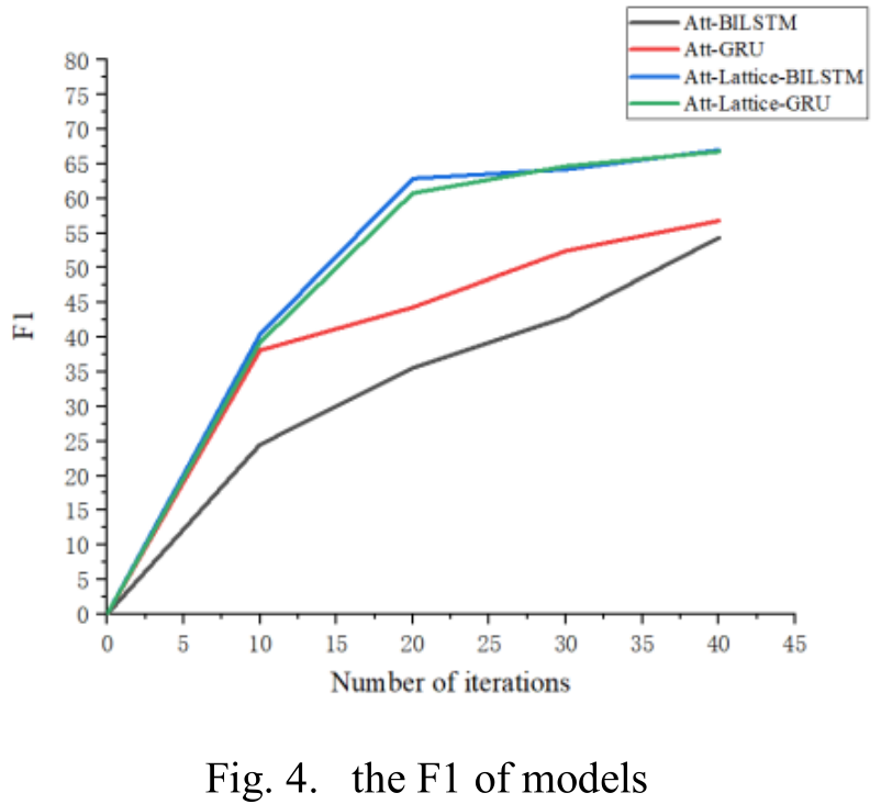
我们也使用相同的服务器来训练这些型号，服务器的配置是：Turbo3.6GHZ，GTX1060Ti，16gram。两种模型的F1和精度结果无明显差异。我们可以观察图6中的时间对比图。

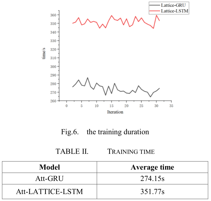
从结果图可以看出，格点单元lattice cells的引入提高了整体模型的性能，每次迭代的平均时间如表2所示。可以改进的是，我们的模型具有更好的性能。

V.  CONCLUTIONS

在这篇文章中，我们引入了一个格结构，可以利用单词信息到经典的关系抽取模型中。这种结构首先匹配字典，获得句子中的潜在单词，然后将这些单词作为新的输入单元。在网络层之后，我们还加入了基于字符的注意机制来提取句子级特征。针对LSTM网络训练时间长的问题，我们采用GRU代替LSTM。最后，在不同的数据集上与其他模型进行比较，得到了较好的实验结果。

In this article, we introduce a lattice structure that can utilize word information into the classic relation extraction model. This structure first matches the dictionary to obtain potential words in the sentence, then uses the words as new input units. We also add a character-based attention mechanism to extract sentence-level features after the network layer. In view of the long training time of the LSTM network, we use GRU instead of LSTM. Finally, compared with other models on different data sets, this model get better experimental results.