这篇记录的内容来自于Andrew Ng教授在coursera网站上的授课。
1.多元线性回归(multivariate linear regression):
h函数:$h_{\theta}{(x)}=\theta_{0}+\sum_{i=1}^{n}{\theta_{i}x_{i}}$
为方便起见,每个样本的维度都设为n+1维,每一维都向后延一位,第一维是1。
则$$h_{\theta}{(x)}=\sum_{i=0}^{n}{\theta_{i}x_{i}}$$
$$h_{\theta}{(x)}={\theta}^{T}x$$
J函数为平方误差函数。
最小化$\frac{1}{2m}\sum_{i=1}^{m}{(h_{\theta}(x^{(i)})-y^{(i)})^2}$。
多元线性回归的梯度下降法:
$\theta_{i}:=\theta_{i}-\alpha\frac{1}{m}\sum_{j=1}^{m}{(h_{\theta}(x^{(j)})-y^{(j)})}x^{(j)}_{i}$
2.特征缩放(feature scaling):在梯度下降时有时会因为样本的某些特征相差了几个数量级,在一个区域内反复振荡,速度很慢。
让这些特征保持在一个相近的范围内了来提高速度,就是特征缩放。
范围不能太大,也不能太小。这只是一个实践性的结论。
使用特征缩放后的拟合函数来进行预测时,新的样本也要缩放一下。
3.均值归一化(mean normalization):对于特征缩放,考虑$$x^{(i)}:=\frac{x^{(i)}-\mu}{S}$$其中mu是平均值,S是最大值减去最小值,
1.梯度下降中学习率不要太大(发散),不要太小(太慢)。
若要求选取学习率,可以尝试将某些数量级的a试一遍。
学习率太大了:
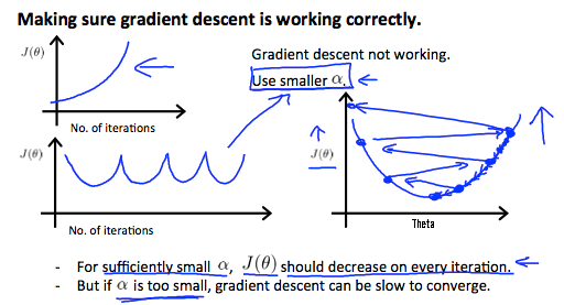
学习率太小了:

1.多项式回归(polynomial regression):$h_{\theta}{(x)}=\sum_{i=0}^{n}{\theta_{i}x_{i}^{i}}$。这里只有一个变量。
2.对于多项式回归,可以变为多元线性回归,但要注意特征缩放。
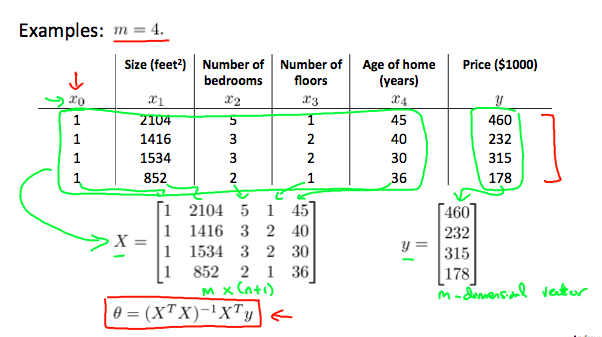
1.标准方程法:多元线性回归的精确解。$\theta=(X^TX)^{-1}X^TY$
Octave:pinv(X'*X)*X'*Y
如何构造X、Y:X为m样本的转置放在一个矩阵中,y就是样本的标签的向量。
证明:http://www.mamicode.com/info-detail-2662773.html
矩阵不可逆?:https://blog.csdn.net/DataAnalyst_ing/article/details/85859226
与梯度下降的比较:样本较少时,标准方程法快;样本较多时,梯度下降快。
标准方程得出的是精确解,梯度下降得出的是近似解。
python实现的多项式回归:
能自动调次数,有均值归一化。


 1 import numpy as np
 2 import pandas as pd
 3 import matplotlib.pyplot as plt
 4 import scipy.optimize as opt
 5 import math
 6 #############################方便起见,一个样本是一行n列的,theta也是一行n列的。
 7 path="ex1data3.txt"
 8 degree=11
 9 ######################################################################代价
10 def cost(theta,x,y):
11     theta=np.matrix(theta)
12     x=np.matrix(x)
13     y=np.matrix(y)
14     z=np.power((x*theta.T-y),2)
15     return np.sum(z)/(2*len(x))###平方误差函数
16 ######################################################################更新函数
17 def gradient(theta,x,y):
18     theta=np.matrix(theta)
19     x=np.matrix(x)
20     y=np.matrix(y)
21     error=x*theta.T-y
22     m=x.shape[0]
23     n=x.shape[1]
24     temp=np.zeros(n)
25     for i in range(n):
26         z=np.multiply(error,x[:,i])
27         temp[i]=np.sum(z)/m###梯度下降
28     return temp
29 ######################################################################处理数据
30 def process(data):
31     x=data.iloc[:,0]
32     now=x
33     data2=pd.DataFrame(np.zeros((data.shape[0],degree)))
34     mean=np.zeros(degree+2)
35     len=np.zeros(degree+2)###n+1项加上输出的1项。
36     for i in range(degree):
37         mean[i+1]=np.mean(now)
38         len[i+1]=now.max()-now.min()+1###计算平均值和差值,+1是防止除0。
39         data2[i]=(now-mean[i+1])/len[i+1]
40         now=now*x
41     x=data.iloc[:,1]
42     mean[degree+1]=np.mean(x)
43     len[degree+1]=x.max()-x.min()+1
44     data2[degree+1]=(x-mean[degree+1])/len[degree+1]
45     mean[0]=1
46     len[0]=1
47     return data2,mean,len
48 ######################################################################决策边界
49 def getBoundary(vector,L,R,mean,len):
50     x=np.linspace(L,R,100)
51     f=np.linspace(L,R,100)
52     for i in range(100):
53         sum=0
54         for j in range(degree+1):
55             k=degree-j
56             if(k==0):
57                 sum+=vector[k]###theta_0不需要变化。
58             else:
59                 sum+=vector[k]*(math.pow(x[i],k)-mean[k])/len[k]
60         f[i]=sum*len[degree+1]+mean[degree+1]###倒推
61     return x,f
62 ######################################################################主函数
63 def main():
64 ################读入数据并处理
65     source=pd.read_csv(path,header=None,names=["population","profit"])
66     data,mean,len=process(source)
67     data.insert(0,"Ones",1)
68     x=np.matrix(data.iloc[:,0:degree+1])
69     y=np.matrix(data.iloc[:,degree+1:degree+2])
70     vector=np.zeros(degree+1)
71 ################梯度下降
72     vector=opt.fmin_tnc(func=cost,x0=vector,fprime=gradient,args=(x,y))[0]
73     print(vector)
74     print(mean)
75     print(len)
76 #################画图
77     x,f=getBoundary(vector,source.population.min(),source.population.max(),mean,len)
78     fig,ax=plt.subplots(figsize=(12,8))###看清楚了
79     ax.plot(x,f,"r",label="prediction")
80     ax.scatter(source.population,source.profit,label="data")
81     ax.set_xlabel("population")
82     ax.set_ylabel("profit")
83     ax.set_title("Polynominal Regression")
84     plt.show()
85 ######################################################################
86 if __name__=="__main__":
87     main()
 posted on

 浙公网安备 33010602011771号