Part I Liner Regression with One Variable

Just a study note for a maching learning course by Andrew Ng

Univariate linear regression

Model Representation

• \(m\): Number of training examples

• \(x^{(i)}\): ”input“ variable / features

• \(y^{(i)}\): ”output“ variable / ”target“ variable

• \((x,y)\) : one training example

• \((x^{(i)},y^{(i)})\) : i-th training example

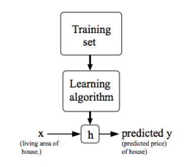
• Function h:
• \(h_\theta(x)=\theta_0+\theta_1x\)

Cost Function

• \(h_\theta(x)=\theta_0+\theta_1x\)
• \(\theta_i\) ：Parameters
• Cost Function : To measure the accuracy of hypothesis function.
• Idea: Choose \(\theta_0,\theta_1\) so that \(h_\theta(x)\) is close to \(y\) for our training example \((x,y)\)
• The Squared Error Function :

\[\ J(\theta_0,\theta_1)=\frac{1}{2m}\sum^{m}_{i=1}(h_\theta(x^{(i)})-y^{(i)})^2 \]

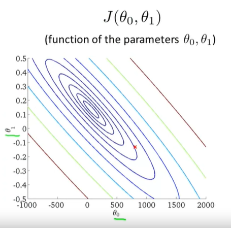
• Goal : \(minimize\ J(\theta_0,\theta_1)\)
• Contour Plot:

Gradient descent

• To \(min\) \(J(\theta_0,\theta_1)\)
• Outline
  • Start with some \(\theta_0,\theta_1\) (\(\theta_0=0,\theta_1=0\))
  • Keeping changing \(\theta_0,\theta_1\) to reduce \(J(\theta_0,\theta_1)\) until we hopefully end up at a minimum.

• The distance between each 'star' in the graph above represents a step determined by our parameter \(\alpha\). A smaller \(\alpha\) would result in a smaller step and a larger \(\alpha\) results in a larger step.

• The direction in which the step is taken is determined by the partial derivative of \(J(\theta_0,\theta_1)\)

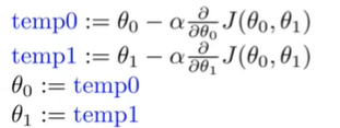
• Gradient descent algorithm

  • repeat until convergence
  \[\theta_j:=\theta_j-\alpha\frac{\partial}{\partial\theta_j}{J(\theta_0,\theta_1)} (\mbox{for}\ j=0\ and\ j=1) \]

  • \(:=\) assign,differ from \(=\)

  • \(\alpha\) : constant value,"learning rate"

  • "simultaneous update:"

    

• To simply the question, we make the question only one parameter \(\theta_1\)

• \(\theta_1:=\theta_1-\alpha\frac{d}{d\theta_1}J(\theta_1)\)

• \(\theta_1\) eventually converges to its minimum value

• We should adjust our parameter \(\alpha\) to ensure that the gradient descent algorithm converges in a reasonable time.

  • If \(\alpha\) is too small, gradient descent can be slow
  • If \(\alpha\) is too large, gradient descent can overshoot the minimum. It may fail to converge, or even diverge.

• When \(\theta_1\) at local optima, \(\frac{d}{d\theta_1}J(\theta_1)=0\)

• As we approach a local minimum, gradient descent will automatically take smaller steps.

• Consider the question with two parameters \(\theta_0,\theta_1\)

• \(\frac{\partial}{\partial\theta_j}{J(\theta_0,\theta_1)}=\frac{\partial}{\partial\theta_j}\frac{1}{2m}\sum^{m}_{i=1}(h(x^{(i)})-y^{(i)})^2=\frac{\partial}{\partial\theta_j}\frac{1}{2m}\sum^{m}_{i=1}(\theta_0+\theta_1x^{(i)}-y^{(i)})^2\)

• \(j=0:\frac{\partial}{\partial\theta_0}J(\theta_0,\theta_1)=\frac{1}{m}\sum^{m}_{i=1}(h(x^{(i)})-y^{(i)})\)

• \(j=1:\frac{\partial}{\partial\theta_1}J(\theta_0,\theta_1)=\frac{1}{m}\sum^{m}_{i=1}(h(x^{(i)})-y^{(i)})x^{(i)}\)

• so we have

\[\theta_0:=\theta_0-\alpha\frac{1}{m}\sum^{m}_{i=1}(h(x^{(i)})-y^{(i)})\\ \theta_1=\theta_1-\alpha\frac{1}{m}\sum^{m}_{i=1}(h(x^{(i)})-y^{(i)})x^{(i)} \]

• the optimization problem we have posed here for linear regression has only one global, and no other local, optima.
• thus gradient descent always converges (assuming the learning rate α is not too large) to the global minimum. Indeed, J is a convex quadratic function.