kaggle竞赛 使用TPU对104种花朵进行分类 第十八次尝试 99.9%准确率 中文注释【深度学习TPU+Keras+Tensorflow+EfficientNetB7】
目录
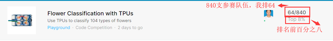
排行榜分数
该排行榜的计算结果约为测试数据的70%。最终结果将基于其他30%,因此最终排名可能会有所不同。(就是排行榜的计算结果不一定等于你的验证集准确率)
第18次尝试的排行榜分数为95.7%,当时我还挺开心的,可能这就是无知者最快乐吧,还好我不知道我自己菜,哈哈哈,但是被大佬喷了,然后我就又加油去学习其他模型,去调参数。

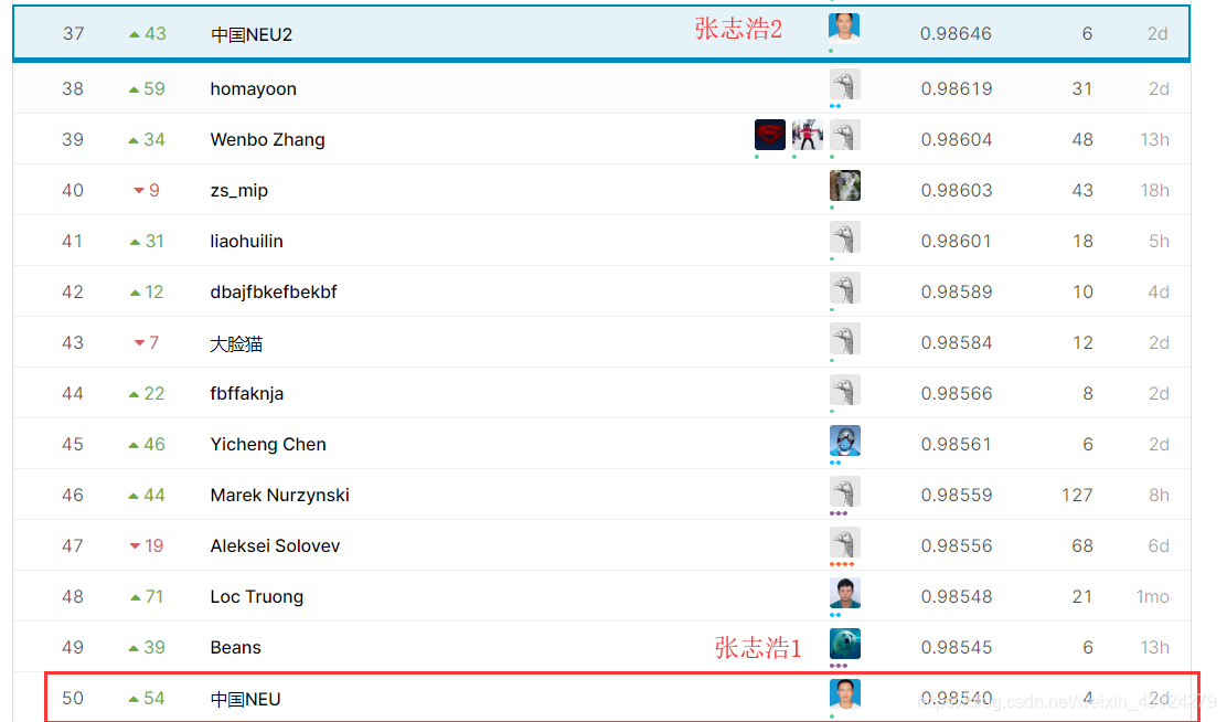
应大佬要求先贴一个第19次尝试(版本19)的排名,正在慢慢进步,别问我为啥名字不一样,因为每个账号一只能提交5次结果,每个账号一周只能用30小时TPU,所以我申请了4个账号,从张志浩1-张志浩4

第20次尝试

第21次尝试

这是第21版本的其他提交分数,深度学习嘛,本来每次训练结果都不一样

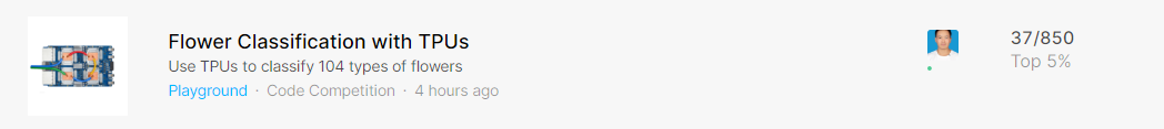
最终排名
我上面的版本21就是最终版本,而且在拿到64名的名次以后我没有再进行训练和提交,最终排名中的37名的分数就是我原来的64名分数

翻译:比赛已经结束。 该排行榜反映了初步的最终排名。 竞赛组织者验证结果后,结果将成为最终结果。
我猜想最终分数与我们之前看到的额不同有两个原因:
1.很多人用与测试集相关的数据集训练,被判定为作弊
2. 比赛最终分数由70%给定的测试集(我们能拿到的test数据)和30%其他测试集决定,我们模型可能在这70%上表现好,在另外30%就差了
比赛过后的一点心得
这个比赛花费了我将近一周的时间,这一周基本都是熬夜熬夜熬夜,哈哈哈哈😂😂😂。
因为这个比赛真的学到好多东西啊,可能因为以前掌握的东西太少了吧。学习了两大莫模型DenseNet+EfficientNet。学习了管道(Pipelining)性能优化、并行读取数据、缓存(cache)性能优化。以前因为数据集小、神经网络简单,从没有考虑过优化。
这次比赛我这几天应该不会再次去尝试了,我参加这次比赛是想把它作为我们学校《深度学习导论》课程的结课作业,已经开始写报告了,写了40多页了,大家有需要就私聊我吧😁😁😁,QQ3382885270,我是菜鸡,而且贼喜欢问别人问题,得到很多大佬的帮助(尤其是经常去烦我们老师,被老师询问为什么老是纠结一些小细节,哈哈哈,还挺有意思的。感谢徐老师😎😎😎),所以我很想能为其他人提供帮助,能和其他人一起变优秀。✨✨✨
心得:
- 该比赛需要梯子,你使用TPU需要验证手机号,验证手机号需要梯子;你使用Kaggle的Kernel也需要梯子。你读取Kaggle数据还是需要梯子。
- 一个账号一周只能使用30小时TPU,一个账号一周只能进行5次结果提交,我建议大家申请很多账号同时参加比赛。而且每次训练模型都需要2小时甚至更多,所以我建议大家同时开多个浏览器,每个浏览器登陆不同账号,同时进行模型的训练,这样2小时就能同时训练很多个模型了。
- 坚持吧兄弟,你会变强。不是只有你很累,没有什么怀才不遇,只是你太菜了。如果你真的很努力很努力,你会开花结果的。
前言
大家好,我是爱做梦的鱼(因为喜欢幻想,总是想象各种美好的事),我是东北大学大三的小菜鸡,非常渴望优秀,羡慕优秀的人,已拿两个暑假offer(拿的大数据开发,因为数据分析的实习岗位不面向本科生,但是还是很喜欢数据分析,我把数据分析当作我仅存的浪漫),
刚系统学习两周深度学习(通过看书《Python深度学习》+《神经网络和深度学习》),欢迎大家找我进行交流😂😂😂
这是我的博客地址:子浩的博客https://blog.csdn.net/weixin_43124279
本次kaggle竞赛地址:https://www.kaggle.com/c/flower-classification-with-tpus/overview
其他文章:
【深度学习 TPU、tensorflow】kaggle竞赛 使用TPU对104种花朵进行分类 第一次尝试 40%准确率
【深度学习TPU+Keras+Tensorflow+EfficientNetB7】kaggle竞赛 使用TPU对104种花朵进行分类 第十八次尝试 99.9%准确率(英文版)
专栏:
深度学习
本竞赛英文全称
Flower Classification with TPUs
Use TPUs to classify 104 types of flowers
以下为比赛的描述:
在这场比赛中,您面临的挑战是建立一个机器学习模型,该模型可识别图像
数据集中的花朵类型(为简单起见,我们坚持使用100多种类型的花朵)。
数据集:
12753个训练图像,3712个验证图像,7382个未标记的测试图像
选用的数据为:
在这次比赛中,我们根据来自五个不同公共数据集的花卉图像对104种花卉进行分类。有些种类非常狭窄,只包含一个特定的花的子种类(例如粉红报春花),而其他种类包含许多子种类(例如野生玫瑰)。
这种竞赛的不同之处在于以TFRecord格式提供图像。 TFRecord格式是Tensorflow中经常使用的容器格式,用于对数据数据文件进行分组和分片以获得最佳训练性能。每个文件都包含许多图像的id,标签(样本数据,用于训练数据)和img(数组形式的实际像素)信息。
- train/*.tfrec-训练集,包括标签。
- val/*.tfrec-验证集。预分割训练样本,带有帮助检查您的模型在TPU上的性能的标签。这种分割是按标签分层的。
- test/*.tfrec-测试集,不带标签的样本-您将预测这些花属于哪一类。
- sample_submission.csv-格式正确的示例提交文件
- id-每个样本的唯一id。
- 标记(在训练数据中)样本所代表的花的类别
版本更新情况
以下准确率全都是验证准确率,和比赛提交以后的准确率有一定区别,因为算法不一样
- V1:官方给出的代码,用了VGG模型,准确率40%
- V2-V8:不断增删层,并调超参数,更换损失函数与优化器 准确率增长到60%就遇到瓶颈了
- V9:尝试通过仅在5分钟内训练softmax层来预热,然后再释放所有重量。准确率下降到50%
- V10:更多数据扩充 准确率55%
- V11:使用LR Scheduler 准确率62%
- V12:同时使用训练和验证数据来训练模型。 准确率68%
- V13;使用谷歌开源新模型 EfficientNetB7 准确率91%,害怕
- V14:训练更长的时间(25个轮次)。准确率82%,下降了,是因为过拟合吧
- V15:回到20个轮次; Global Max Pooling instead of Average。(全局最大池而不是平均。) 准确率67%,不适合
- V16:回滚到global average pooling (全局平均池) 准确率81%
- V18:回滚到V13,并调节部分参数 准确率99.9%,恐怖如斯,我好无敌
1. 安装efficientnet
!pip install -q efficientnet #因为我们想用 EfficientNet模型,所以我们先进行安装efficientnet,
# 感叹号表示调用控制台,这句代码等价于于在控制台输入了pip install -q efficientnet
2. 导入需要的包
# 导入需要的包
import math, re, os # math:包括一些通用的数学公式;re:字符串正则匹配;os:操作系统接口
import tensorflow as tf # tensorflow包
import numpy as np # numpy操作数组
from matplotlib import pyplot as plt   # matplotlib进行画图
from kaggle_datasets import KaggleDatasets # Kaggle数据集
import efficientnet.tfkeras as efn    # 导入efficientnet模型
# 从python的sklearn机器学习中导入f1值、精度、召回率和混淆矩阵
from sklearn.metrics import f1_score, precision_score, recall_score, confusion_matrix

print("Tensorflow version " + tf.__version__) #检查tensorflow的版本
Tensorflow version 2.1.0
3. 检测TPU和GPU
我这里注释掉的原因是我们已经知道TPU和GPU存在,而且我们打算完全用TPU而不用GPU
# Detect hardware, return appropriate distribution strategy
# try:
      # TPU检测。 如果设置了TPU_NAME环境变量,则不需要任何参数。 在Kaggle上,情况总是如此。
#     tpu = tf.distribute.cluster_resolver.TPUClusterResolver()
#     print('Running on TPU ', tpu.master())
# except ValueError:
#     tpu = None

# if tpu:
#     tf.config.experimental_connect_to_cluster(tpu)
#     tf.tpu.experimental.initialize_tpu_system(tpu)
#     strategy = tf.distribute.experimental.TPUStrategy(tpu)
# else:
#     strategy = tf.distribute.get_strategy() # default distribution strategy in Tensorflow. Works on CPU and single GPU.

# print("REPLICAS: ", strategy.num_replicas_in_sync) #输出副本数
4. 配置TPU、访问路径等
AUTO = tf.data.experimental.AUTOTUNE # 可以让程序自动的选择最优的线程并行个数

# Create strategy from tpu
# 从TPU创建部署
tpu = tf.distribute.cluster_resolver.TPUClusterResolver() #如果先前设置好了TPU_NAME环境变量,不需要再给参数.
tf.config.experimental_connect_to_cluster(tpu) # 配置实验连接到群集
tf.tpu.experimental.initialize_tpu_system(tpu) # 初始化tpu系统
strategy = tf.distribute.experimental.TPUStrategy(tpu) # 设置TPU部署


# 官方给出的竞赛数据访问注释
# Competition data access
# TPUs read data directly from Google Cloud Storage (GCS).
# This Kaggle utility will copy the dataset to a GCS bucket co-located with the TPU.
# If you have multiple datasets attached to the notebook,
# you can pass the name of a specific dataset to the get_gcs_path function.
# The name of the dataset is the name of the directory it is mounted in.
# Use !ls /kaggle/input/ to list attached datasets.
# 比赛数据访问
# TPU直接从Google Cloud Storage(GCS)读取数据。
# 该Kaggle实用程序会将数据集复制到与TPU并置的GCS存储桶中。
# 如果笔记本有多个数据集,
# 您可以将特定数据集的名称传递给get_gcs_path函数。
# 数据集的名称是其安装目录的名称。
# 使用!ls / kaggle / input /列出附加的数据集。

GCS_DS_PATH = KaggleDatasets().get_gcs_path() #设置Kaggle数据的访问路径

# Configuration

IMAGE_SIZE = [512, 512] # 配置像素点矩阵大小
EPOCHS = 20 # # 配置模型训练的轮次
BATCH_SIZE = 16 * strategy.num_replicas_in_sync # 设置每个小批量的大小
# 配置不同大小图片的路径
GCS_PATH_SELECT = { # available image sizes
    192: GCS_DS_PATH + '/tfrecords-jpeg-192x192',
    224: GCS_DS_PATH + '/tfrecords-jpeg-224x224',
    331: GCS_DS_PATH + '/tfrecords-jpeg-331x331',
    512: GCS_DS_PATH + '/tfrecords-jpeg-512x512'
}
GCS_PATH = GCS_PATH_SELECT[IMAGE_SIZE[0]]

TRAINING_FILENAMES = tf.io.gfile.glob(GCS_PATH + '/train/*.tfrec') # 训练集路径
VALIDATION_FILENAMES = tf.io.gfile.glob(GCS_PATH + '/val/*.tfrec') # 验证集路径
TEST_FILENAMES = tf.io.gfile.glob(GCS_PATH + '/test/*.tfrec') # 测试集路径 predictions on this dataset should be submitted for the competition
# 104种花的名称
CLASSES = ['pink primrose',    'hard-leaved pocket orchid', 'canterbury bells', 'sweet pea',     'wild geranium',     'tiger lily',           'moon orchid',              'bird of paradise', 'monkshood',        'globe thistle',         # 00 - 09
           'snapdragon',       "colt's foot",               'king protea',      'spear thistle', 'yellow iris',       'globe-flower',         'purple coneflower',        'peruvian lily',    'balloon flower',   'giant white arum lily', # 10 - 19
           'fire lily',        'pincushion flower',         'fritillary',       'red ginger',    'grape hyacinth',    'corn poppy',           'prince of wales feathers', 'stemless gentian', 'artichoke',        'sweet william',         # 20 - 29
           'carnation',        'garden phlox',              'love in the mist', 'cosmos',        'alpine sea holly',  'ruby-lipped cattleya', 'cape flower',              'great masterwort', 'siam tulip',       'lenten rose',           # 30 - 39
           'barberton daisy',  'daffodil',                  'sword lily',       'poinsettia',    'bolero deep blue',  'wallflower',           'marigold',                 'buttercup',        'daisy',            'common dandelion',      # 40 - 49
           'petunia',          'wild pansy',                'primula',          'sunflower',     'lilac hibiscus',    'bishop of llandaff',   'gaura',                    'geranium',         'orange dahlia',    'pink-yellow dahlia',    # 50 - 59
           'cautleya spicata', 'japanese anemone',          'black-eyed susan', 'silverbush',    'californian poppy', 'osteospermum',         'spring crocus',            'iris',             'windflower',       'tree poppy',            # 60 - 69
           'gazania',          'azalea',                    'water lily',       'rose',          'thorn apple',       'morning glory',        'passion flower',           'lotus',            'toad lily',        'anthurium',             # 70 - 79
           'frangipani',       'clematis',                  'hibiscus',         'columbine',     'desert-rose',       'tree mallow',          'magnolia',                 'cyclamen ',        'watercress',       'canna lily',            # 80 - 89
           'hippeastrum ',     'bee balm',                  'pink quill',       'foxglove',      'bougainvillea',     'camellia',             'mallow',                   'mexican petunia',  'bromelia',         'blanket flower',        # 90 - 99
           'trumpet creeper',  'blackberry lily',           'common tulip',     'wild rose']
5. 各种函数
5.1. 可视化函数
# 展示训练和验证曲线,也就是损失和准确率随轮次的变化
def display_training_curves(training, validation, title, subplot):
    if subplot%10==1: # set up the subplots on the first call # 在第一次调用该函数时设置子图
        plt.subplots(figsize=(10,10), facecolor='#F0F0F0')
        plt.tight_layout()
    ax = plt.subplot(subplot) #设置子图
    ax.set_facecolor('#F8F8F8') #设置背景颜色
    ax.plot(training) #画训练集的曲线
    ax.plot(validation) #画测试集的曲线
    ax.set_title('model '+ title)
    ax.set_ylabel(title) #设置y轴标题
    #ax.set_ylim(0.28,1.05)
    ax.set_xlabel('epoch') #设置x轴标题
    ax.legend(['train', 'valid.']) #设置图例

# 绘制混淆矩阵
def display_confusion_matrix(cmat, score, precision, recall):
    plt.figure(figsize=(15,15))  # 设置画布大小
    ax = plt.gca() #返回当前axes(matplotlib.axes.Axes) 获取当前子图
    ax.matshow(cmat, cmap='Reds') #绘制矩阵
    ax.set_xticks(range(len(CLASSES)))  #根据花朵类别数(其实就是104)设置x轴范围
    ax.set_xticklabels(CLASSES, fontdict={'fontsize': 7}) #设置x轴下标字体的大小
    plt.setp(ax.get_xticklabels(), rotation=45, ha="left", rotation_mode="anchor") #更换x轴下标角度
    ax.set_yticks(range(len(CLASSES)))  #根据花朵类别数(其实就是104)设置y轴范围
    ax.set_yticklabels(CLASSES, fontdict={'fontsize': 7}) #设置y轴下标字体的大小
    plt.setp(ax.get_yticklabels(), rotation=45, ha="right", rotation_mode="anchor") #更换y轴下标角度
    titlestring = ""
    if score is not None:
        titlestring += 'f1 = {:.3f} '.format(score) #更改格式为有3位小数的浮点数
    if precision is not None:
        titlestring += '\nprecision = {:.3f} '.format(precision) #更改格式为有3位小数的浮点数
    if recall is not None:
        titlestring += '\nrecall = {:.3f} '.format(recall) #更改格式为有3位小数的浮点数
    if len(titlestring) > 0:
        ax.text(101, 1, titlestring, fontdict={'fontsize': 18, 'horizontalalignment':'right', 'verticalalignment':'top', 'color':'#804040'}) #添加文本注释
    plt.show()
# 设置numpy数组基本属性,设置显示15个数字,用于插入换行符的每行字符数(默认为75)。
# threshold : int, optional,Total number of array elements which trigger summarization rather than full repr (default 1000).
# 当数组数目过大时,设置显示几个数字,其余用省略号
# linewidth : int, optional,The number of characters per line for the purpose of inserting line breaks (default 75).
# 用于插入换行符的每行字符数(默认为75)。
np.set_printoptions(threshold=15, linewidth=80)

# 将小批量图片和标签处理为numpy向量格式
def batch_to_numpy_images_and_labels(data):
    images, labels = data
    numpy_images = images.numpy() #将图像转换为numpy向量格式
    numpy_labels = labels.numpy() #将label标签转换为numpy向量格式
    if numpy_labels.dtype == object: # 在这种情况下为二进制字符串,它们是图像ID字符串
        numpy_labels = [None for _ in enumerate(numpy_images)]
    # 如果没有标签,只有图像ID,则对标签返回None(测试数据就是这种情况)
    return numpy_images, numpy_labels

# 把实际类型和模型预测出来的模型一起显示在图片上方,这是用给验证集的,当对验证集预测完标签后和验证集的实际标签进行比较
# label,图片中花朵的实际类别
# correct_label,当前我们预测的类别
def title_from_label_and_target(label, correct_label):
    # 如果没有预测的类别,则返回实际类别,比如训练集
    if correct_label is None:
        return CLASSES[label], True
    correct = (label == correct_label) #判断一下实际类别和我们预测的类别是否一致
    # 如果一致,则返回OK,不一致则返回NO加实际类别
    return "{} [{}{}{}]".format(CLASSES[label], 'OK' if correct else 'NO', u"\u2192" if not correct else '',
                                CLASSES[correct_label] if not correct else ''), correct

# 绘制一朵花
def display_one_flower(image, title, subplot, red=False, titlesize=16):
    plt.subplot(*subplot)
    plt.axis('off') # 不显示坐标尺寸
    plt.imshow(image) #函数负责对图像进行处理,并显示其格式;而plt.show()则是将plt.imshow()处理后的函数显示出来。
    if len(title) > 0:
        #绘制图片的标题
        plt.title(title, fontsize=int(titlesize) if not red else int(titlesize/1.2), color='red' if red else 'black',
                  fontdict={'verticalalignment':'center'}, pad=int(titlesize/1.5))
    return (subplot[0], subplot[1], subplot[2]+1)

# 展示小批量图片,我们在下面的代码中经常展示20张照片
def display_batch_of_images(databatch, predictions=None):
    """This will work with:
    display_batch_of_images(images)   # 只展示图片 测试集需要这个
    display_batch_of_images(images, predictions) #展示图片加预测的类别 测试集需要这个
    display_batch_of_images((images, labels)) #展示图片加实际标签 训练集需要这个
    display_batch_of_images((images, labels), predictions) #展示图片+实际类别+预测类别 验证集需要这个,因为验证集既有实际标签,也会进行预测
    """
    # 读取图片和实际标签数据,而且这些数据被转换成numpy向量的格式
    images, labels = batch_to_numpy_images_and_labels(databatch)
    # 如果没有实际标签(即if labels is None为true),比如测试集,那么我们需要将labels变量设为每个元素都为none
    if labels is None:
        labels = [None for _ in enumerate(images)]

    # 自动平方:这将删除不适合正方形或矩形的数据
    rows = int(math.sqrt(len(images)))
    cols = len(images)//rows  #" // " 表示整数除法,返回不大于结果的一个最大的整数,向下取整

    # 大小和间距
    FIGSIZE = 13.0  #画图大小
    SPACING = 0.1
    subplot=(rows,cols,1)
    if rows < cols:
        # 如果行大于列
        plt.figure(figsize=(FIGSIZE,FIGSIZE/cols*rows))
    else:
        plt.figure(figsize=(FIGSIZE/rows*cols,FIGSIZE))

    # display
    for i, (image, label) in enumerate(zip(images[:rows*cols], labels[:rows*cols])):
        title = '' if label is None else CLASSES[label]
        correct = True
        if predictions is not None:
            title, correct = title_from_label_and_target(predictions[i], label)
        dynamic_titlesize = FIGSIZE*SPACING/max(rows,cols)*40+3 # 经过测试可以在1x1到10x10图像上工作的魔术公式
        subplot = display_one_flower(image, title, subplot, not correct, titlesize=dynamic_titlesize)

    #layout
    plt.tight_layout()
    if label is None and predictions is None:
        plt.subplots_adjust(wspace=0, hspace=0)
    else:
        plt.subplots_adjust(wspace=SPACING, hspace=SPACING)
    plt.show()
5.2. 数据集函数
# 准备图像数据
def decode_image(image_data):
    image = tf.image.decode_jpeg(image_data, channels=3) # 将图片解码
    # 之前训练图像保存在一个 uint8 类型的数组中,取值区间为 [0, 255]。我们需要将其变换为一个 float32 数组,其形取值范围为 0~1。
    # 将图片转换为[0,1]范围内的浮点数
    image = tf.cast(image, tf.float32) / 255.0
    image = tf.reshape(image, [*IMAGE_SIZE, 3]) # TPU所需的精确的大小
    return image

# 读取带有标签的TFRecord 格式文件
def read_labeled_tfrecord(example):
    LABELED_TFREC_FORMAT = {
        "image": tf.io.FixedLenFeature([], tf.string), # tf.string means bytestring
        "class": tf.io.FixedLenFeature([], tf.int64),  # shape [] means single element
    }
    example = tf.io.parse_single_example(example, LABELED_TFREC_FORMAT)
    image = decode_image(example['image'])
    label = tf.cast(example['class'], tf.int32)
    return image, label # returns a dataset of (image, label) pairs

# 读取没有标签的TFRecord 格式文件
def read_unlabeled_tfrecord(example):
    UNLABELED_TFREC_FORMAT = {
        "image": tf.io.FixedLenFeature([], tf.string), # tf.string means bytestring
        "id": tf.io.FixedLenFeature([], tf.string),  # shape [] means single element
        # class is missing, this competitions's challenge is to predict flower classes for the test dataset
    }
    example = tf.io.parse_single_example(example, UNLABELED_TFREC_FORMAT)
    image = decode_image(example['image'])
    idnum = example['id']
    return image, idnum # returns a dataset of image(s)

# 加载数据集
# 这三个参数分别为:文件路径、是否有标签、是否按顺序(就是要不要把数据顺序打乱)
def load_dataset(filenames, labeled=True, ordered=False):
    # 从TFRecords读取。 为了获得最佳性能,请一次从多个文件中读取数据,而不考虑数据顺序。 顺序无关紧要,因为无论如何我们都会对数据进行混洗。
    ignore_order = tf.data.Options()
    if not ordered:
        ignore_order.experimental_deterministic = False # 禁用顺序,提高速度

    dataset = tf.data.TFRecordDataset(filenames, num_parallel_reads=AUTO)  # 自动交错读取多个文件
    dataset = dataset.with_options(ignore_order) # 在流入数据后立即使用数据,而不是按原始顺序使用
    dataset = dataset.map(read_labeled_tfrecord if labeled else read_unlabeled_tfrecord, num_parallel_calls=AUTO)
    # 如果标记为True则返回(图像,label)对的数据集,如果标记为False,则返回(图像,id)对的数据集
    return dataset

# 按水平 (从左向右) 随机翻转图像.返回图片的参数image和label
def data_augment(image, label, seed=2020):
    # TensorFlow函数:tf.image.random_flip_left_right
    # 按水平 (从左向右) 随机翻转图像.
    # 以1比2的概率,输出image沿着第二维翻转的内容,即,width.否则按原样输出图像.
    # 参数:
    # image:形状为[height, width, channels]的三维张量.
    # seed:一个Python整数,用于创建一个随机种子.查看tf.set_random_seed行为.
    # 返回:一个与image具有相同类型和形状的三维张量.
    image = tf.image.random_flip_left_right(image, seed=seed)

#     image = tf.image.random_flip_up_down(image, seed=seed)
#     image = tf.image.random_brightness(image, 0.1, seed=seed)
#     image = tf.image.random_jpeg_quality(image, 85, 100, seed=seed)
#     image = tf.image.resize(image, [530, 530])
#     image = tf.image.random_crop(image, [512, 512], seed=seed)
    #image = tf.image.random_saturation(image, 0, 2)
    return image, label

# 获取训练集
def get_training_dataset():
    # 加载训练集,第一个参数为训练集路径,第二个参数表示有标签
    dataset = load_dataset(TRAINING_FILENAMES, labeled=True)
    # 将数据转换并行化
    # 为num_parallel_calls 参数选择最佳值取决于您的硬件、训练数据的特征(例如其大小和形状)、Map 功能的成本以及在 CPU 上同时进行的其他处理;
    dataset = dataset.map(data_augment, num_parallel_calls=AUTO)
    # 重复此数据集count次数
    # 函数形式:repeat(count=None)
    # 参数count:(可选)表示数据集应重复的次数。默认行为(如果count是None或-1)是无限期重复的数据集。
    dataset = dataset.repeat() # 数据集必须重复几个轮次
    dataset = dataset.shuffle(2048) #将数据打乱,括号中数值越大,混乱程度越大
    dataset = dataset.batch(BATCH_SIZE) # 按照顺序将小批量中样本数目行数据合成一个小批量,最后一个小批量可能小于20
    # pipeline(管道)读取数据,在训练时预取下一批(自动调整预取缓冲区大小)
    dataset = dataset.prefetch(AUTO)
    return dataset

# 获取验证集
def get_validation_dataset(ordered=False):
    # 加载训练集,第一个参数为验证集路径,第二个参数表示有标签,第三个参数为不按照顺序
    dataset = load_dataset(VALIDATION_FILENAMES, labeled=True, ordered=ordered)
    dataset = dataset.batch(BATCH_SIZE) ## 按照顺序将小批量中样本数目行数据合成一个小批量,最后一个小批量可能小于20
    dataset = dataset.cache() # 使用.cache()方法:当计算缓存空间足够时,将preprocess的数据存储在缓存空间中将大幅提高计算速度。
    # pipeline(管道)读取数据,在训练时预取下一批(自动调整预取缓冲区大小)
    dataset = dataset.prefetch(AUTO)
    return dataset

# 将训练集和验证集合并
def get_train_valid_datasets():
    dataset = load_dataset(TRAINING_FILENAMES + VALIDATION_FILENAMES, labeled=True)
       # 将数据转换并行化
    # 加载训练集,第一个参数为训练集路径,第二个参数表示有标签
    dataset = dataset.map(data_augment, num_parallel_calls=AUTO)
    # 重复此数据集count次数
    # 函数形式:repeat(count=None)
    # 参数count:(可选)表示数据集应重复的次数。默认行为(如果count是None或-1)是无限期重复的数据集。
    dataset = dataset.repeat() # 数据集必须重复几个轮次
    dataset = dataset.shuffle(2048) # 将数据打乱,括号中数值越大,混乱程度越大
    dataset = dataset.batch(BATCH_SIZE)
    # pipeline(管道)读取数据,在训练时预取下一批(自动调整预取缓冲区大小)
    dataset = dataset.prefetch(AUTO)
    return dataset

# 获取测试集
def get_test_dataset(ordered=False):
    dataset = load_dataset(TEST_FILENAMES, labeled=False, ordered=ordered)
    dataset = dataset.batch(BATCH_SIZE)
    # pipeline(管道)读取数据,在训练时预取下一批(自动调整预取缓冲区大小)
    dataset = dataset.prefetch(AUTO)
    return dataset

# 计算数据集样本数目
def count_data_items(filenames):
    # 数据集的数量以.tfrec文件的名称编写,即flowers00-230.tfrec = 230个数据项
    n = [int(re.compile(r"-([0-9]*)\.").search(filename).group(1)) for filename in filenames]
    return np.sum(n)
5.3. 模型函数
# LearningRate Function 自己编写的学习率函数
# 返回学习率·
def lrfn(epoch):
    LR_START = 0.00001 # 初始学习率
    LR_MAX = 0.00005 * strategy.num_replicas_in_sync # 最大学习率
    LR_MIN = 0.00001 # 最小学习率
    LR_RAMPUP_EPOCHS = 5
    LR_SUSTAIN_EPOCHS = 0
    LR_EXP_DECAY = .8

    if epoch < LR_RAMPUP_EPOCHS:
        lr = (LR_MAX - LR_START) / LR_RAMPUP_EPOCHS * epoch + LR_START
    elif epoch < LR_RAMPUP_EPOCHS + LR_SUSTAIN_EPOCHS:
        lr = LR_MAX
    else:
        lr = (LR_MAX - LR_MIN) * LR_EXP_DECAY**(epoch - LR_RAMPUP_EPOCHS - LR_SUSTAIN_EPOCHS) + LR_MIN
    return lr
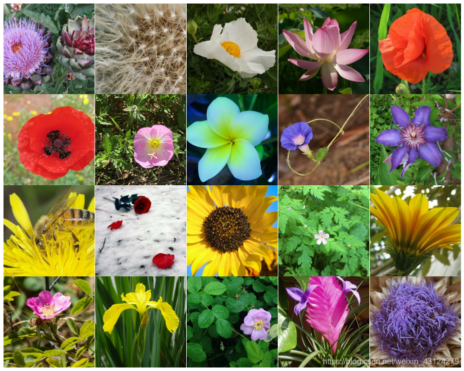
6. 数据集可视化
# 数据展示
print("Training data shapes:")
# 输出训练集前3个小批量的图像数据形状、标签形状
for image, label in get_training_dataset().take(3):
    print(image.numpy().shape, label.numpy().shape)
# 训练数据标签示例
print("Training data label examples:", label.numpy())

print("Validation data shapes:")
# 输出验证集前3个小批量的图像数据形状、标签形状
for image, label in get_validation_dataset().take(3):
    print(image.numpy().shape, label.numpy().shape)
# 验证数据标签示例
print("Validation data label examples:", label.numpy())

print("Test data shapes:")
# 输出测试集前3个小批量的图像数据形状、标签形状
for image, idnum in get_test_dataset().take(3):
    print(image.numpy().shape, idnum.numpy().shape)
# 测试集的id示例
print("Test data IDs:", idnum.numpy().astype('U')) # U=unicode string
Training data shapes:
(128, 512, 512, 3) (128,)
(128, 512, 512, 3) (128,)
(128, 512, 512, 3) (128,)
Training data label examples: [ 1  7 49 ... 77 53 67]
Validation data shapes:
(128, 512, 512, 3) (128,)
(128, 512, 512, 3) (128,)
(128, 512, 512, 3) (128,)
Validation data label examples: [49  4 91 ... 66 93 21]
Test data shapes:
(128, 512, 512, 3) (128,)
(128, 512, 512, 3) (128,)
(128, 512, 512, 3) (128,)
Test data IDs: ['75d255458' '8d1bc9b54' 'ff30e8b96' ... '256e89fc6' 'f6482ab55' '82f95de55']
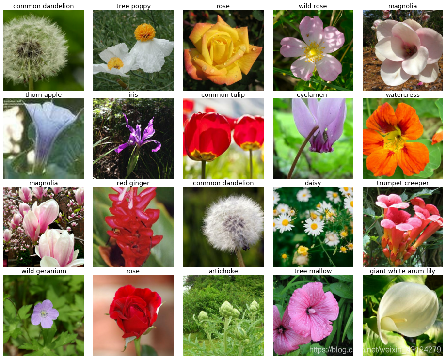
# 查看训练集
training_dataset = get_training_dataset() #通过一个函数来获取训练集
training_dataset = training_dataset.unbatch().batch(20) # 将训练集分成大小为20的小批量
train_batch = iter(training_dataset) # 首先获得Iterator对象
# 再次运行该单元格以获取下一组图像
display_batch_of_images(next(train_batch))
# 查看测试集
test_dataset = get_test_dataset() #通过一个函数来获取测试集
test_dataset = test_dataset.unbatch().batch(20) # 将训练集分成大小为20的小批量
test_batch = iter(test_dataset) # 首先获得Iterator对象
# 再次运行该单元格以获取下一组图像
display_batch_of_images(next(test_batch))
7. 训练模型
NUM_TRAINING_IMAGES = count_data_items(TRAINING_FILENAMES) # 训练集样本数目
NUM_VALIDATION_IMAGES = count_data_items(VALIDATION_FILENAMES) # 验证集样本数目
NUM_TEST_IMAGES = count_data_items(TEST_FILENAMES) # 测试集样本数目
STEPS_PER_EPOCH = NUM_TRAINING_IMAGES // BATCH_SIZE # 每轮次中的步数=训练集样本数除以每个小批量中样本数目
# 输出训练集、验证集和测试集的数目
print('Dataset: {} training images, {} validation images, {} unlabeled test images'.format(NUM_TRAINING_IMAGES, NUM_VALIDATION_IMAGES, NUM_TEST_IMAGES))
Dataset: 12753 training images, 3712 validation images, 7382 unlabeled test images
7.1. 创建模型并加载到TPU
# 创建模型并加载到TPU
with strategy.scope():
    # 创建EfficientNetB7模型
    enet = efn.EfficientNetB7( # 选择EfficientNet中的EfficientNetB7模型
        input_shape=(512, 512, 3), # 规定输入数据的形状
        weights='imagenet', # 用ImageNet的参数初始化模型的参数。如果不想使用ImageNet上预训练到的权重初始话模型,可以将各语句的中'imagenet'替换为'None'。
        include_top=False # include_top:是否保留顶层的3个全连接网络,False为不保留
    )

    # 创建模型
    model = tf.keras.Sequential([ #Sequential类(仅用于层的线性堆叠,这是目前最常见的网络架构)
        enet, # EfficientNetB7模型
        tf.keras.layers.GlobalAveragePooling2D(), #全局平均池
        # len(CLASSES):表示这个层将返回一个大小为类别个数(104)的张量
        # activation='softmax':表示这个层将返回图片在104个类别上的概率,其中最大的概率表示这个图片的预测类别
        # softmax激活函数的本质就是将一个K维的任意实数向量压缩(映射)成另一个K维的实数向量,其中向量中的每个元素取值都介于(0,1)之间并且和为1。
        # 在多分类单标签问题中,可以用softmax作为最后的激活层,取概率最高的作为结果
        tf.keras.layers.Dense(len(CLASSES), activation='softmax')
    ])

    # 编译模型
    model.compile(
        optimizer=tf.keras.optimizers.Adam(), #优化器:Adam 是一种可以替代传统随机梯度下降(SGD)过程的一阶优化算法,它能基于训练数据迭代地更新神经网络权重
        # 损失函数:
        # 对于多分类问题,可以用分类交叉熵(categorical crossentropy)或稀疏分类交叉熵(sparse_categorical_crossentropy)损失函数
        # 这个sparse_categorical_crossentropy损失函数在数学上与 categorical_crossentropy 完全相同,
        # 如果目标是 one-hot 编码的,那么使用 categorical_crossentropy 作为损失;
        # 如果目标是整数,那么使用 sparse_categorical_crossentropy 作为损失。
        loss = 'sparse_categorical_crossentropy',
        metrics=['sparse_categorical_accuracy'] # 监控指标:分类准确率
    )

     #模型的摘要
    model.summary()
Downloading data from https://github.com/Callidior/keras-applications/releases/download/efficientnet/efficientnet-b7_weights_tf_dim_ordering_tf_kernels_autoaugment_notop.h5
258441216/258434480 [==============================] - 4s 0us/step
Model: "sequential"
_________________________________________________________________
Layer (type)                 Output Shape              Param #
=================================================================
efficientnet-b7 (Model)      (None, 16, 16, 2560)      64097680
_________________________________________________________________
global_average_pooling2d (Gl (None, 2560)              0
_________________________________________________________________
dense (Dense)                (None, 104)               266344
=================================================================
Total params: 64,364,024
Trainable params: 64,053,304
Non-trainable params: 310,720
_________________________________________________________________
保存全模型
可以对整个模型进行保存,其保存的内容包括:
- 该模型的架构
- 模型的权重(在训练期间学到的)
- 模型的训练配置(你传递给编译的),如果有的话
- 优化器及其状态(如果有的话)(这使您可以从中断的地方重新启动训练
model.save('the_save_model.h5') #保存全模型
7.2. 训练模型
# scheduler = tf.keras.callbacks.ReduceLROnPlateau(patience=3, verbose=1)
# 作为回调函数的一员,LearningRateScheduler 可以按照epoch的次数自动调整学习率,
# 参数:
# schedule:一个函数,它将一个epoch索引作为输入(整数,从0开始索引)并返回一个新的学习速率作为输出(浮点数)。
# 我们这里用lrfn(epoch)函数
# verbose:int;当其为0时,保持安静;当其为1时,表示更新消息。
lr_schedule = tf.keras.callbacks.LearningRateScheduler(lrfn, verbose=1)

# 训练模型
history = model.fit(
    get_train_valid_datasets(),  # 获取训练集
    steps_per_epoch=STEPS_PER_EPOCH, # 设置每轮的步数
    epochs=EPOCHS,  # 设置轮次
    callbacks=[lr_schedule], # 设置回调函数
    validation_data=get_validation_dataset() # 设置验证集
)
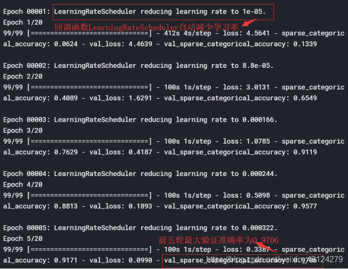
Train for 99 steps
Epoch 00001: LearningRateScheduler reducing learning rate to 1e-05.
Epoch 1/20
99/99 [==============================] - 412s 4s/step - loss: 4.5641 - sparse_categorical_accuracy: 0.0624 - val_loss: 4.4639 - val_sparse_categorical_accuracy: 0.1339
Epoch 00002: LearningRateScheduler reducing learning rate to 8.8e-05.
Epoch 2/20
99/99 [==============================] - 100s 1s/step - loss: 3.0131 - sparse_categorical_accuracy: 0.4089 - val_loss: 1.6291 - val_sparse_categorical_accuracy: 0.6549
Epoch 00003: LearningRateScheduler reducing learning rate to 0.000166.
Epoch 3/20
99/99 [==============================] - 100s 1s/step - loss: 1.0785 - sparse_categorical_accuracy: 0.7629 - val_loss: 0.4187 - val_sparse_categorical_accuracy: 0.9119
Epoch 00004: LearningRateScheduler reducing learning rate to 0.000244.
Epoch 4/20
99/99 [==============================] - 100s 1s/step - loss: 0.5098 - sparse_categorical_accuracy: 0.8813 - val_loss: 0.1893 - val_sparse_categorical_accuracy: 0.9577
Epoch 00005: LearningRateScheduler reducing learning rate to 0.000322.
Epoch 5/20
99/99 [==============================] - 100s 1s/step - loss: 0.3387 - sparse_categorical_accuracy: 0.9171 - val_loss: 0.0990 - val_sparse_categorical_accuracy: 0.9706
Epoch 00006: LearningRateScheduler reducing learning rate to 0.0004.
Epoch 6/20
99/99 [==============================] - 100s 1s/step - loss: 0.2712 - sparse_categorical_accuracy: 0.9316 - val_loss: 0.0653 - val_sparse_categorical_accuracy: 0.9811
Epoch 00007: LearningRateScheduler reducing learning rate to 0.000322.
Epoch 7/20
99/99 [==============================] - 100s 1s/step - loss: 0.1728 - sparse_categorical_accuracy: 0.9566 - val_loss: 0.0263 - val_sparse_categorical_accuracy: 0.9935
Epoch 00008: LearningRateScheduler reducing learning rate to 0.0002596000000000001.
Epoch 8/20
99/99 [==============================] - 100s 1s/step - loss: 0.1122 - sparse_categorical_accuracy: 0.9716 - val_loss: 0.0147 - val_sparse_categorical_accuracy: 0.9954
Epoch 00009: LearningRateScheduler reducing learning rate to 0.00020968000000000004.
Epoch 9/20
99/99 [==============================] - 100s 1s/step - loss: 0.0762 - sparse_categorical_accuracy: 0.9815 - val_loss: 0.0073 - val_sparse_categorical_accuracy: 0.9976
Epoch 00010: LearningRateScheduler reducing learning rate to 0.00016974400000000002.
Epoch 10/20
99/99 [==============================] - 100s 1s/step - loss: 0.0535 - sparse_categorical_accuracy: 0.9878 - val_loss: 0.0039 - val_sparse_categorical_accuracy: 0.9987
Epoch 00011: LearningRateScheduler reducing learning rate to 0.00013779520000000003.
Epoch 11/20
99/99 [==============================] - 100s 1s/step - loss: 0.0404 - sparse_categorical_accuracy: 0.9907 - val_loss: 0.0026 - val_sparse_categorical_accuracy: 0.9995
Epoch 00012: LearningRateScheduler reducing learning rate to 0.00011223616000000004.
Epoch 12/20
99/99 [==============================] - 101s 1s/step - loss: 0.0355 - sparse_categorical_accuracy: 0.9912 - val_loss: 0.0024 - val_sparse_categorical_accuracy: 0.9995
Epoch 00013: LearningRateScheduler reducing learning rate to 9.178892800000003e-05.
Epoch 13/20
99/99 [==============================] - 100s 1s/step - loss: 0.0292 - sparse_categorical_accuracy: 0.9936 - val_loss: 0.0023 - val_sparse_categorical_accuracy: 0.9992
Epoch 00014: LearningRateScheduler reducing learning rate to 7.543114240000003e-05.
Epoch 14/20
99/99 [==============================] - 100s 1s/step - loss: 0.0241 - sparse_categorical_accuracy: 0.9950 - val_loss: 0.0020 - val_sparse_categorical_accuracy: 0.9997
Epoch 00015: LearningRateScheduler reducing learning rate to 6.234491392000002e-05.
Epoch 15/20
99/99 [==============================] - 100s 1s/step - loss: 0.0231 - sparse_categorical_accuracy: 0.9950 - val_loss: 0.0012 - val_sparse_categorical_accuracy: 1.0000
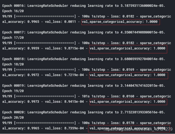
Epoch 00016: LearningRateScheduler reducing learning rate to 5.1875931136000024e-05.
Epoch 16/20
99/99 [==============================] - 100s 1s/step - loss: 0.0182 - sparse_categorical_accuracy: 0.9965 - val_loss: 0.0011 - val_sparse_categorical_accuracy: 1.0000
Epoch 00017: LearningRateScheduler reducing learning rate to 4.3500744908800015e-05.
Epoch 17/20
99/99 [==============================] - 100s 1s/step - loss: 0.0182 - sparse_categorical_accuracy: 0.9959 - val_loss: 9.8715e-04 - val_sparse_categorical_accuracy: 1.0000
Epoch 00018: LearningRateScheduler reducing learning rate to 3.6800595927040014e-05.
Epoch 18/20
99/99 [==============================] - 100s 1s/step - loss: 0.0169 - sparse_categorical_accuracy: 0.9972 - val_loss: 9.7219e-04 - val_sparse_categorical_accuracy: 1.0000
Epoch 00019: LearningRateScheduler reducing learning rate to 3.1440476741632015e-05.
Epoch 19/20
99/99 [==============================] - 101s 1s/step - loss: 0.0160 - sparse_categorical_accuracy: 0.9973 - val_loss: 8.9415e-04 - val_sparse_categorical_accuracy: 1.0000
Epoch 00020: LearningRateScheduler reducing learning rate to 2.7152381393305616e-05.
Epoch 20/20
99/99 [==============================] - 100s 1s/step - loss: 0.0170 - sparse_categorical_accuracy: 0.9965 - val_loss: 8.7359e-04 - val_sparse_categorical_accuracy: 1.0000
第1-5轮。我们发现回调函数LearningRateScheduler自动调整学习率,并且验证准确率最大为0.9706
最后的五轮,第16-20轮。我们发现回调函数LearningRateScheduler自动调整学习率,并且验证准确率保持在1
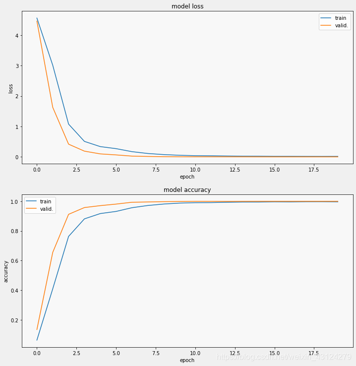
7.3. 绘制损失和准确率曲线
# 画出训练集和验证集随轮次变化的损失和准确率
display_training_curves(history.history['loss'], history.history['val_loss'], 'loss', 211) #损失曲线
display_training_curves(history.history['sparse_categorical_accuracy'], history.history['val_sparse_categorical_accuracy'], 'accuracy', 212) #准确率曲线
# display_training_curves(history.history['loss'], history.history['loss'], 'loss', 211)
# display_training_curves(history.history['sparse_categorical_accuracy'], history.history['sparse_categorical_accuracy'], 'accuracy', 212)
7.4. 绘制混淆矩阵
# 因为我们要分割数据集并分别对图像和标签进行迭代,所以顺序很重要。
cmdataset = get_validation_dataset(ordered=True)  # 验证集
images_ds = cmdataset.map(lambda image, label: image)  # 图像集
labels_ds = cmdataset.map(lambda image, label: label).unbatch() # 标签集
cm_correct_labels = next(iter(labels_ds.batch(NUM_VALIDATION_IMAGES))).numpy() # get everything as one batch
cm_probabilities = model.predict(images_ds) # 图片在104个类别上的概率
cm_predictions = np.argmax(cm_probabilities, axis=-1) # 其中最大的概率表示这个图片的预测类别
print("Correct   labels: ", cm_correct_labels.shape, cm_correct_labels) # 输出正确(实际)标签的形状、输出正确标签
print("Predicted labels: ", cm_predictions.shape, cm_predictions) # 输出预测标签的形状、输出预测标签
Correct   labels:  (3712,) [ 50  13  74 ... 102  48  67]
Predicted labels:  (3712,) [ 50  13  74 ... 102  48  67]
# 计算混淆矩阵
# 参数为实际标签和预测的标签
cmat = confusion_matrix(cm_correct_labels, cm_predictions, labels=range(len(CLASSES)))
# 计算f1分数
score = f1_score(cm_correct_labels, cm_predictions, labels=range(len(CLASSES)), average='macro')
# 计算精确率
precision = precision_score(cm_correct_labels, cm_predictions, labels=range(len(CLASSES)), average='macro')
# 计算召回率
recall = recall_score(cm_correct_labels, cm_predictions, labels=range(len(CLASSES)), average='macro')
# 归一化
cmat = (cmat.T / cmat.sum(axis=1)).T # normalized
# 绘制混淆矩阵
display_confusion_matrix(cmat, score, precision, recall)
# 输出f1分数、精确率、召回率
print('f1 score: {:.3f}, precision: {:.3f}, recall: {:.3f}'.format(score, precision, recall))
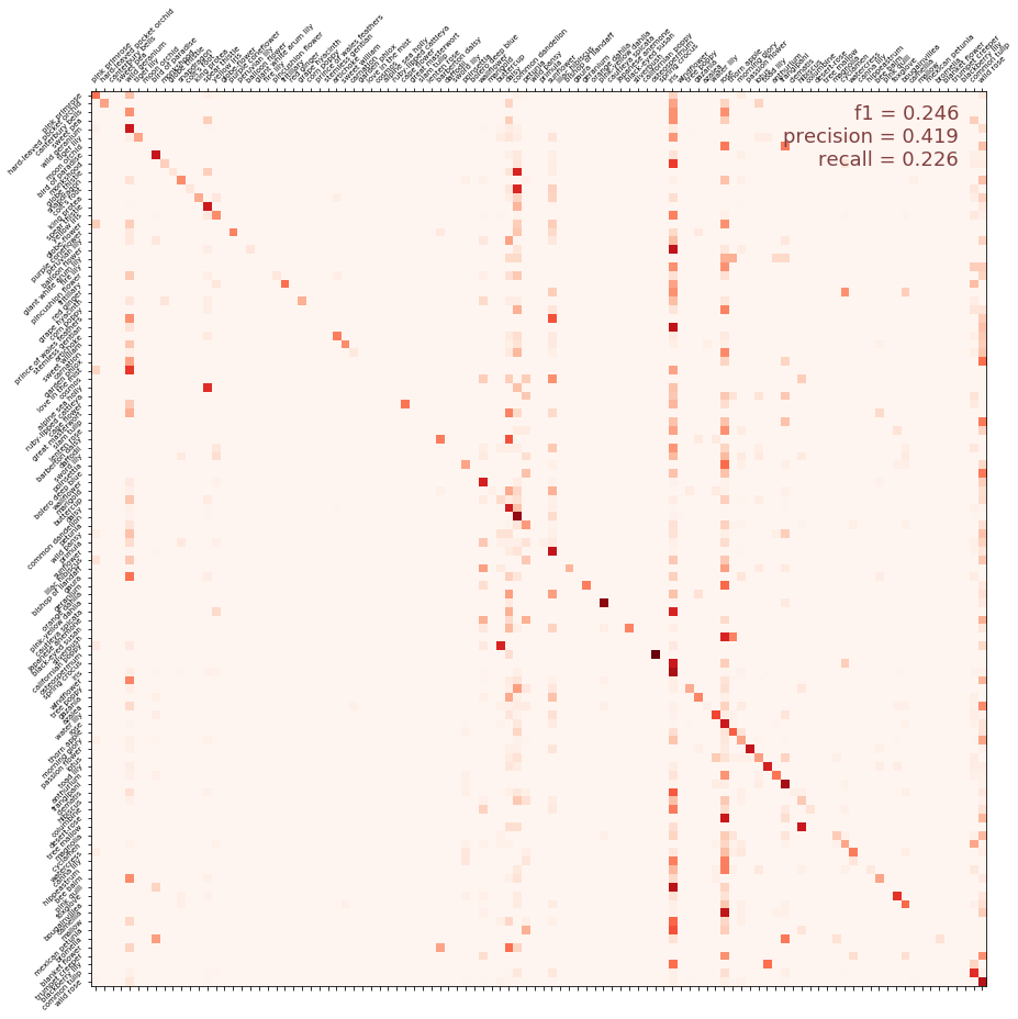
图一:非本次的混沌矩阵,这是V1版本的混沌矩阵,这里放图只是因为我们最后的准确率(V18版本)太高,图一无法让我们感受到混淆矩阵的魅力。贴一个准确率低一点的来让我们感受混淆矩阵的魅力。
对验证集预测后,
准确率(accuracy )为40%
f1分数(f1 score)=0.246,
精确率(precision)=0.419,
召回率(recall)=0.226
图二:本次的混沌矩阵,这是V18版本的混沌矩阵,
对验证集预测后,
准确率(accuracy )为99.9%
f1分数(f1 score)=1,
精确率(precision)=1,
召回率(recall)=1
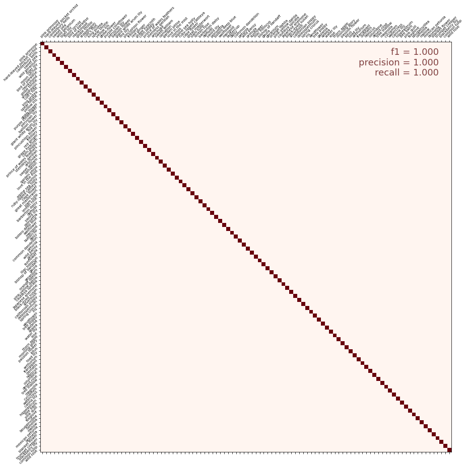
f1 score: 1.000, precision: 1.000, recall: 1.000
8. 预测
# 因为我们要分割数据集并分别对图像和ID进行迭代,所以顺序很重要。
test_ds = get_test_dataset(ordered=True) # 测试集

# 对测试集进行预测
print('Computing predictions...')
test_images_ds = test_ds.map(lambda image, idnum: image) #测试集的图片
probabilities = model.predict(test_images_ds) # 图片在104个类别上的概率
predictions = np.argmax(probabilities, axis=-1) # 其中最大的概率表示这个图片的预测类别
print(predictions) # 输出预测类别

# 生成提交文件
print('Generating submission.csv file...')
test_ids_ds = test_ds.map(lambda image, idnum: idnum).unbatch() #测试集的id
test_ids = next(iter(test_ids_ds.batch(NUM_TEST_IMAGES))).numpy().astype('U') # 准换id的数据类型 # all in one batch

# 第一种存储文件方式,不需要pandas
# np.savetxt('submission.csv', np.rec.fromarrays([test_ids, predictions]), fmt=['%s', '%d'], delimiter=',', header='id,label', comments='')
# 第二种存储文件的方式,需要pandas
import pandas as pd
test = pd.DataFrame({"id":test_ids,"label":predictions}) #将id列和label列创建成一个DataFrame
print(test.head) # 输出test的前几行
test.to_csv("submission.csv",index = False) # 生成没有索引的submission.csv,以便提交
Computing predictions...
[ 67  28  83 ...  86 102  62]
Generating submission.csv file...
<bound method NDFrame.head of              id  label
0     252d840db     67
1     1c4736dea     28
2     c37a6f3e9     83
3     00e4f514e    103
4     59d1b6146     70
...         ...    ...
7377  c785abe6f      7
7378  9b9c0e574     68
7379  e46998f4d     86
7380  523df966b    102
7381  e86e2a592     62

[7382 rows x 2 columns]>
9. 视觉上进行一下验证,看下预测效果
这里为什么选择验证集进行视觉上的验证?
我们选取验证集进行验证,因为模型是根据训练集训练的,而验证集和测试集都和训练集毫不相关,但是验证集有实际标签,方便我们进行验证
dataset = get_validation_dataset()  # 获取验证集
dataset = dataset.unbatch().batch(20)  #将验证集分成大小为20的小批量
batch = iter(dataset) # 将数据集转化为Iterator对象
# 再次运行该单元格以获取下一组图像
images, labels = next(batch) # 获取验证集的下一个批量
probabilities = model.predict(images) # 图片在104个类别上的概率
predictions = np.argmax(probabilities, axis=-1) # 其中最大的概率表示这个图片的预测类别
display_batch_of_images((images, labels), predictions) # 展示一个批量的图片,图片标题为预测标签+预测标签是否正确(OK或NO)
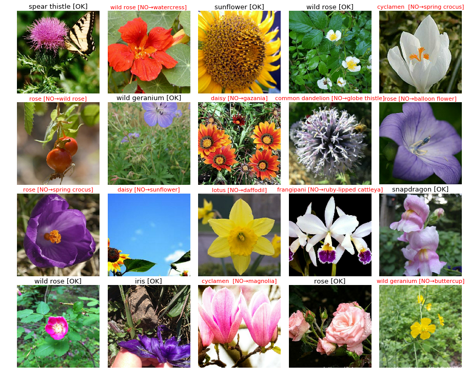
# 举个例子:标题为wild rose(NO->watercress),这个图片实际是豆瓣花,但是预测为野玫瑰,所以它是错的。所以它的标签为 野玫瑰(NO->豆瓣花)
图一:非本次的经过预测的验证集部分图片,这是V1版本,这里放图只是因为我们最后的准确率(V18版本)太高,图一无法让我们看到预测失败时的情况。
对验证集预测后,
准确率(accuracy )为40%
f1分数(f1 score)=0.246,
精确率(precision)=0.419,
召回率(recall)=0.226
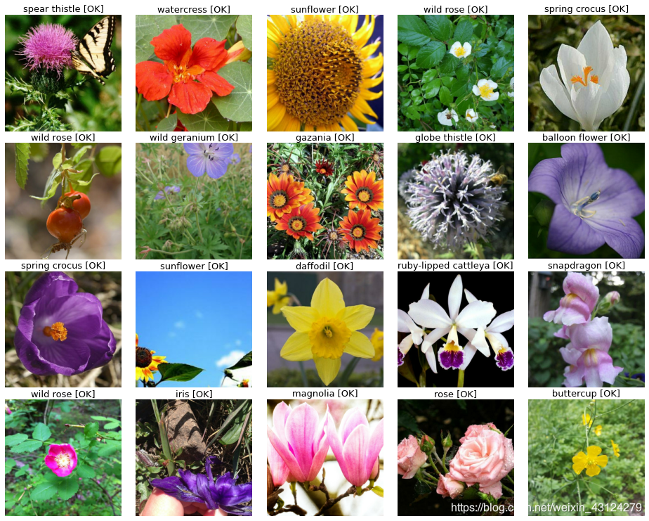
图二:本次的经过预测的验证集的部分图片,这是V18版本,对验证集预测后的
准确率(accuracy )为99.9%
f1分数(f1 score)=1,
精确率(precision)=1,
召回率(recall)=1

 浙公网安备 33010602011771号