UFLDL深度学习笔记 (七)拓扑稀疏编码与矩阵化
UFLDL深度学习笔记 (七)拓扑稀疏编码与矩阵化
主要思路
前面几篇所讲的都是围绕神经网络展开的,一个标志就是激活函数非线性;在前人的研究中,也存在线性激活函数的稀疏编码,该方法试图直接学习数据的特征集,利用与此特征集相应的基向量,将学习得到的特征集从特征空间转换到样本数据空间,这样可以用特征集重构样本数据。
数据集、特征集、基向量分别表示为\(x、A、s\).构造如下目标代价函数,对估计误差的代价采用二阶范数,对稀疏性因子的惩罚代价采用一阶范数。原文中没有对误差项在数据集上做平均,真实情况下都会除以数据集个数\(m\).
接下来,原文中解释说为了增强稀疏性约束,避免取\(A\)的缩放值也能获得相同的代价,稀疏性惩罚需要考虑特征集的数值,进一步改进代价函数为
代价函数仍然存在L1范数的0点不可微问题,通过近似平滑解决,定义常量值平滑参数\(\epsilon\), 将代价函数变成
由于本代价函数非凸,而固定任意一个变量之后,代价函数是凸函数,所以可以通过交替固定\(A,s\)来求最优化代价的\(A,s\). 理论上对上式最优化取得的特征集与通过稀疏自编码学习得到的特征集差不多,人类视觉神经具有一种特点,大脑皮层 V1 区神经元能够按特定的方向对边缘进行检测,同时,这些神经元(在生理上)被组织成超柱(hypercolumns),在超柱中,相邻神经元以相似的方向对边缘进行检测,一个神经元检测水平边缘,其相邻神经元检测到的边缘就稍微偏离水平方向。为了使算法达到这种 拓扑性 ,也就是说相邻的特征激活具有一定连续性、平滑性,我们将惩罚项也改造成考虑相邻特征值,在2X2分组情况下,把原来 \(\sqrt{s_{1,1}^2+\epsilon}\)这一项换成 \(\sqrt{s_{1,1}^2+s_{1,2}^2+s_{2,1}^2 +s_{2,2}^2+ \epsilon}\) 。得到拓扑稀疏编码的代价函数为
进一步用分组矩阵G来表示邻域分组规则,\(G_{r,c}=1\)表示第r组包含第c个特征,目标函数重写为
矩阵化推导
以上符号都是非常抽象意义上的变量,矩阵化实现时就需要考虑清楚每行每列的操作是不是按照预设的每一项运算规则实现的,原文中没有这部分内容,我也花费了一番功夫推导。
按照前文所说的交替求\(A,s\)最优化策略,我们需要先推导代价函数对\(A,s\)的偏导。设定矩阵表示展开为\(A=[_{Wj,f}]_{visibleSize \times featureSize}\). \(s=[S_{Wj,f}]_{featureSize\times m}\). 令\(V=visibleSize, F=featureSize\).
固定\(s\)求解\(A\)的梯度与最优取值
代价的一阶范数项对\(A\)求偏导为0.
单向合并成矩阵表示为
同时我们发现此表达式为一阶方程,可以得到代价函数取极小值时的\(A\)。可得s固定时使代价函数最小的\(A\)为
即$$min J(A,s) \Leftrightarrow A = \frac {xs^T} {ssT+m \gamma I}; $$ .
固定\(A\)求解\(s\)的梯度
展开代价函数并对\(s\)求解,
其中\(G=[g_{l,f}]_{F \times F}\) ,\(g_{l,f}=1\)表示第\(l\)组包含第f个特征。 S_smooth表示根据拓扑编码要求,对特征值的邻域进行平滑后的特征矩阵。
进行矩阵化改写,可以得到,两个求和式可以分别写成矩阵乘法:
这个矩阵表达式不能得到使代价函数最小的\(S\)解析式,这个最优化过程需要使用迭代的方式获得,可以使用梯度下降这类最优化方法。
至此我们得到了编写代码需要的所有矩阵化表达。
代码实现
在本节实践实例中,主文件是 sparseCodingExercise.m ,对\(A,s\)的代价梯度计算模块分别是 sparseCodingWeightCost.m、sparseCodingFeatureCost.m. 按照上述矩阵推导分别填充其中的公式部分,全部代码见https://github.com/codgeek/deeplearning。
分别固定\(A,s\)进行最优化的步骤在sparseCodingExercise.m中,有几条需要注意的地方,否则将会很难训练出结果。
- 每次交替开始前,不能随机设定特征值,而是设定为
featureMatrix = weightMatrix'*batchPatches; - 加载原始图像的函数
sampleIMAGES.m中不能调用归一化normalizeData。和稀疏自编码不同。 - 前面推导的固定\(s\)时最优化\(A\)表示中千万不能漏掉单位矩阵,是\(\gamma\)乘以单位矩阵,不能直接加\(\gamma\)。公式为
weightMatrix = (batchPatches*(featureMatrix'))/(featureMatrix*(featureMatrix')+gamma*batchNumPatches*eye(numFeatures));.
两个梯度公式代码如下。
function [cost, grad] = sparseCodingWeightCost(weightMatrix, featureMatrix, visibleSize, numFeatures,  patches, gamma, lambda, epsilon, groupMatrix)
%sparseCodingWeightCost - given the features in featureMatrix,
%                         computes the cost and gradient with respect to
%                         the weights, given in weightMatrix
% parameters
%   weightMatrix  - the weight matrix. weightMatrix(:, c) is the cth basis
%                   vector.
%   featureMatrix - the feature matrix. featureMatrix(:, c) is the features
%                   for the cth example
%   visibleSize   - number of pixels in the patches
%   numFeatures   - number of features
%   patches       - patches
%   gamma         - weight decay parameter (on weightMatrix)
%   lambda        - L1 sparsity weight (on featureMatrix)
%   epsilon       - L1 sparsity epsilon
%   groupMatrix   - the grouping matrix. groupMatrix(r, :) indicates the
%                   features included in the rth group. groupMatrix(r, c)
%                   is 1 if the cth feature is in the rth group and 0
%                   otherwise.
    if exist('groupMatrix', 'var')
        assert(size(groupMatrix, 2) == numFeatures, 'groupMatrix has bad dimension');
    else
        groupMatrix = eye(numFeatures);
    end

    numExamples = size(patches, 2);

    weightMatrix = reshape(weightMatrix, visibleSize, numFeatures);
    featureMatrix = reshape(featureMatrix, numFeatures, numExamples);

    % -------------------- YOUR CODE HERE --------------------
    % Instructions:
    %   Write code to compute the cost and gradient with respect to the
    %   weights given in weightMatrix.
    % -------------------- YOUR CODE HERE --------------------
    linearError = weightMatrix * featureMatrix - patches;
    normError = sum(sum(linearError .* linearError))./numExamples;% 公式中代价项是二阶范数的平方,所以不用在开方
    normWeight = sum(sum(weightMatrix .* weightMatrix));

    topoFeature = groupMatrix*(featureMatrix.*featureMatrix);
    smoothFeature = sqrt(topoFeature + epsilon);
    costFeature = sum(sum(smoothFeature));% L1 范数为sum(|x|),对x加上平滑参数后,sum(sqrt(x2+epsilon)).容易错写为sqrt(sum(x2+epsilon))实际是L2范数

%     cost = normError + gamma.*normWeight;
    cost = normError + lambda.*costFeature + gamma.*normWeight;
    grad = 2./numExamples.*(linearError*featureMatrix') + (2*gamma) .* weightMatrix;
%     grad = 2.*(weightMatrix*featureMatrix - patches)*featureMatrix' + 2.*gamma*weightMatrix;
    grad = grad(:);

end
function [cost, grad] = sparseCodingFeatureCost(weightMatrix, featureMatrix, visibleSize, numFeatures, patches, gamma, lambda, epsilon, groupMatrix)
%sparseCodingFeatureCost - given the weights in weightMatrix,
%                          computes the cost and gradient with respect to
%                          the features, given in featureMatrix
% parameters
%   weightMatrix  - the weight matrix. weightMatrix(:, c) is the cth basis
%                   vector.
%   featureMatrix - the feature matrix. featureMatrix(:, c) is the features
%                   for the cth example
%   visibleSize   - number of pixels in the patches
%   numFeatures   - number of features
%   patches       - patches
%   gamma         - weight decay parameter (on weightMatrix)
%   lambda        - L1 sparsity weight (on featureMatrix)
%   epsilon       - L1 sparsity epsilon
%   groupMatrix   - the grouping matrix. groupMatrix(r, :) indicates the
%                   features included in the rth group. groupMatrix(r, c)
%                   is 1 if the cth feature is in the rth group and 0
%                   otherwise.

    if exist('groupMatrix', 'var')
        assert(size(groupMatrix, 2) == numFeatures, 'groupMatrix has bad dimension');
    else
        groupMatrix = eye(numFeatures);
    end

    numExamples = size(patches, 2);

    weightMatrix = reshape(weightMatrix, visibleSize, numFeatures);
    featureMatrix = reshape(featureMatrix, numFeatures, numExamples);

    linearError = weightMatrix * featureMatrix - patches;
    normError = sum(sum(linearError .* linearError))./numExamples;
    normWeight = sum(sum(weightMatrix .* weightMatrix));
    topoFeature = groupMatrix*(featureMatrix.*featureMatrix);
    smoothFeature = sqrt(topoFeature + epsilon);
    costFeature = sum(sum(smoothFeature));% L1 范数为sum(|x|),对x加上平滑参数后,sum(sqrt(x2+epsilon)).容易错写为sqrt(sum(x2+epsilon))实际是L2范数

    cost = normError + lambda.*costFeature + gamma.*normWeight;
    grad = 2./numExamples.*(weightMatrix' * linearError) + lambda.*featureMatrix.*( (groupMatrix')*(1 ./ smoothFeature) );% 不止(f,i)本项偏导非零,(f-1,i)……,groupMatrix第f列不为0的所有行对应项都有s(f,i)的偏导
    grad = grad(:);
end
训练结果
数据来源还是稀疏自编码一节所用的图片, 设定特征层包含121个节点,输入层为8X8patch即64个节点,拓扑邻域为3X3的方阵,运行200次训练,
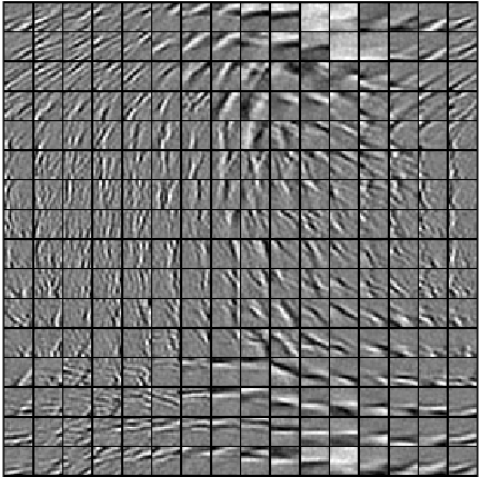
当输入值为对应特征值时,每个激活值会有最大响应,所以把A矩阵每一行的64个向量还原成8*8的图片patch,也就是特征值了,每个隐藏层对应一个,总共121个。结果如下图. 可看出在当前参数下,相同迭代次数,cg算法的图片特征更加清晰。
| lbfgs | cg |
|---|---|
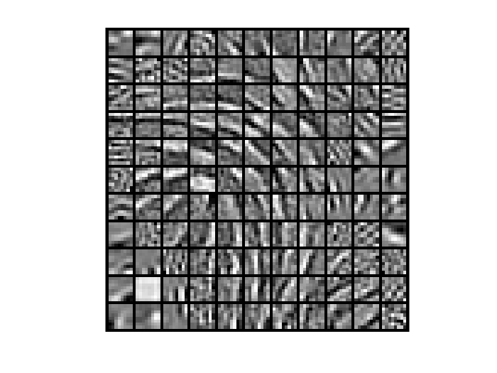 |
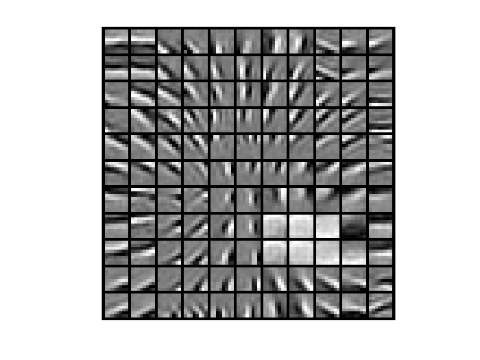 |
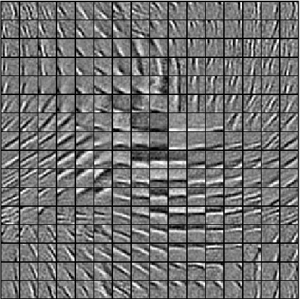
为了看到更精细的训练结果,增加特征层以及输入层节点数,特征层采用256个节点,输入层分别试验了14X14以及15X15,相应需要增加拓扑邻域的大小,采用5X5的方阵。迭代算法采用cg。特征的清晰程度以及拓扑结构的完整性已经和示例中的结果无差别。边缘特征有序排列。而当把输入节点个数增加到16X16, 训练效果出现恶化,边缘特征开始变得模糊,原因也可以理解,特征层已经不再大于输入层,超完备基的条件不成立了,得到的训练效果也相对变差。
| 14X14输入节点,拓扑5X5 | 15X15输入节点,拓扑5X5 |
|---|---|
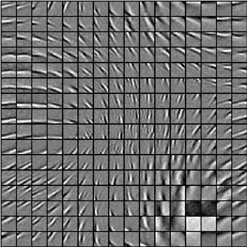 |
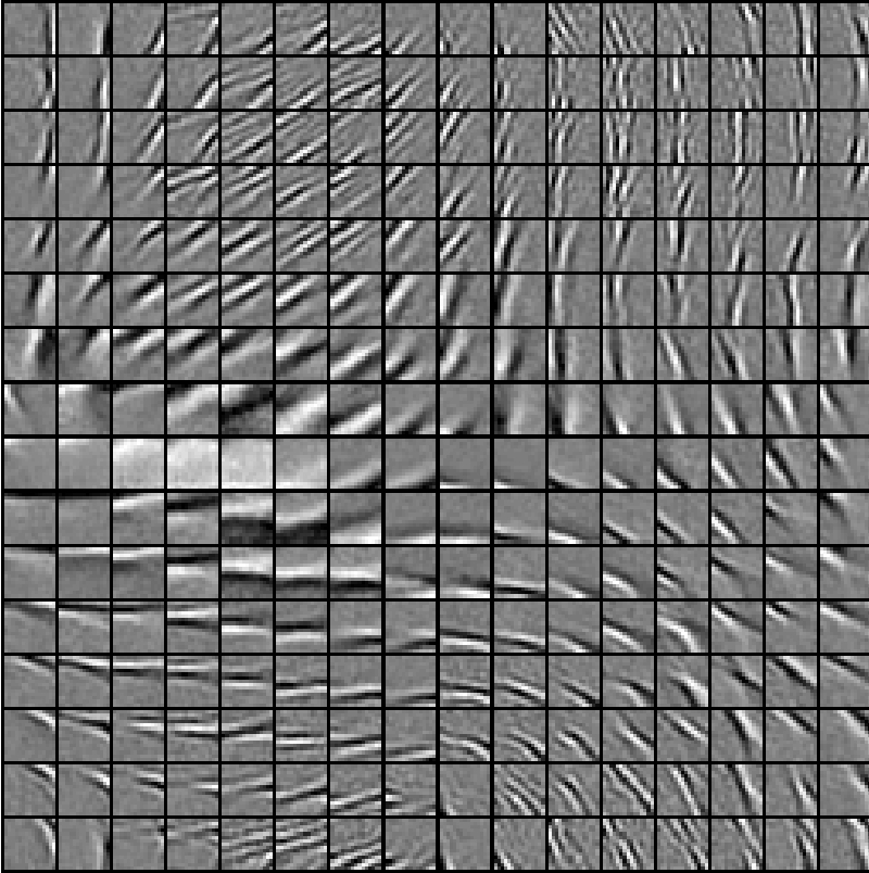 |
增加输入节点的结果:
| 16X16输入节点,拓扑3X3 | 16X16输入节点,拓扑5X5 |
|---|---|
 |
 |

 浙公网安备 33010602011771号