KNN&多项式分类器的设计
KNN 分类器构造
一、KNN 算法的思路:
存在一个样本数据集合,称为训练样本集,且样本集中每个数据都存在标签,即样本集中每一数据与所属分类的对应关系。
输入没有标签的数据后,将新数据中的每个特征与样本集中数据对应的特征进行比较,提取出样本集中特征最相似数据(最近邻)的分类标签。选择 k 个最相似数据中出现次数最多的分类作为新数据的分类。
二、算法步骤:
- 计算未知实例到所有已知实例的距离;
- 选择参数 K;
- 根据多数表决( majority-voting )规则,将未知实例归类为样本中最多数的类别。
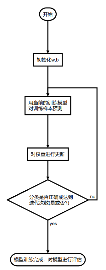
算法流程图
距离的衡量方法
欧拉距离 这种测量方式就是简单的平面几何中两点之间的直线距离。
上述方法延伸至三维或更多维的情况,总结公式为:
曼哈顿距离 ,街区的距离
K 值的选择
K 值的选择会影响结果,如下图:
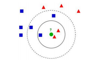
图中的数据集都打好了 label ,一类是蓝色正方形,一类是红色三角形,绿色圆形是待分类的数据。
K = 3 时,范围内红色三角形多,这个待分类点属于红色三角形。
K = 5 时,范围内蓝色正方形多,这个待分类点属于蓝色正方形。
如何选择一个最佳的 K 值取决于数据。一般较大 K 值能减小噪声的影响,但会使类别之间的界限变得模糊。因此 K 的取值一般比较小 ( K < 20 )。
改进:
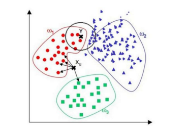
在点 Y 的预测中,范围内三角形类数量占优,因此将 Y 点归为三角形。但从视觉上观测,分为圆形类更合理。根据这种情况,可以在距离测量中加入权重,如 1/d (d: 距离)。
from __future__ import print_function
import sys
import os
import math
import numpy as np
from sklearn import datasets
import matplotlib.pyplot as plt
from collections import Counter
from sklearn.datasets import make_classification


def shuffle_data(X, y, seed=None):
    if seed:
        np.random.seed(seed)
    idx = np.arange(X.shape[0])
    np.random.shuffle(idx)
    return X[idx], y[idx]


# 正规化数据集 X
def normalize(X, axis=-1, p=2):
    lp_norm = np.atleast_1d(np.linalg.norm(X, p, axis))
    lp_norm[lp_norm == 0] = 1
    return X / np.expand_dims(lp_norm, axis)


# 标准化数据集 X
def standardize(X):
    X_std = np.zeros(X.shape)
    mean = X.mean(axis=0)
    std = X.std(axis=0)
    # 分母不能等于 0 的情形
    # X_std = (X - X.mean(axis=0)) / X.std(axis=0)
    for col in range(np.shape(X)[1]):
        if std[col]:
            X_std[:, col] = (X_std[:, col] - mean[col]) / std[col]
    return X_std


# 划分数据集为训练集和测试集
def train_test_split(X, y, test_size=0.2, shuffle=True, seed=None):
    if shuffle:
        X, y = shuffle_data(X, y, seed)
    n_train_samples = int(X.shape[0] * (1 - test_size))
    x_train, x_test = X[:n_train_samples], X[n_train_samples:]
    y_train, y_test = y[:n_train_samples], y[n_train_samples:]
    return x_train, x_test, y_train, y_test


def accuracy(y, y_pred):
    y = y.reshape(y.shape[0], -1)
    y_pred = y_pred.reshape(y_pred.shape[0], -1)
    return np.sum(y == y_pred) / len(y)


class KNN():
    def __init__(self, k=5):
        self.k = k

    # 计算一个样本与训练集中所有样本的欧氏距离的平方
    def euclidean_distance(self, one_sample, X_train):
        one_sample = one_sample.reshape(1, -1)
        X_train = X_train.reshape(X_train.shape[0], -1)
        distances = np.power(np.tile(one_sample, (X_train.shape[0], 1)) - X_train, 2).sum(axis=1)
        return distances

    # 获取 k 个近邻的类别标签
    def get_k_neighbor_labels(self, distances, y_train, k):
        k_neighbor_labels = []
        for distance in np.sort(distances)[:k]:
            label = y_train[distances == distance]
            k_neighbor_labels.append(label)
        return np.array(k_neighbor_labels).reshape(-1, )

    # 进行标签统计,得票最多的标签就是该测试样本的预测标签
    def vote(self, one_sample, X_train, y_train, k):
        distances = self.euclidean_distance(one_sample, X_train)  # print(distances.shape)
        y_train = y_train.reshape(y_train.shape[0], 1)
        k_neighbor_labels = self.get_k_neighbor_labels(distances, y_train, k)  # print(k_neighbor_labels.shape)
        find_label, find_count = 0, 0
        for label, count in Counter(k_neighbor_labels).items():
            if count > find_count:
                find_count = count
                find_label = label
        return find_label

    # 对测试集进行预测
    def predict(self, X_test, X_train, y_train):
        y_pred = []
        for sample in X_test:
            label = self.vote(sample, X_train, y_train, self.k)
            y_pred.append(label)  # print(y_pred)
        return np.array(y_pred)


def main():
    data = make_classification(n_samples=200, n_features=4, n_informative=2,
                               n_redundant=2, n_repeated=0, n_classes=2)
    X, y = data[0], data[1]
    for i in range(2, 200, 3):
        X_train, X_test, y_train, y_test = train_test_split(X, y, test_size=0.33, shuffle=True)
        clf = KNN(k=i)
        y_pred = clf.predict(X_test, X_train, y_train)
        accu = accuracy(y_test, y_pred)
        print("k=", i, "\tAccuracy:", accu)


if __name__ == "__main__": main()
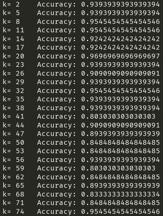
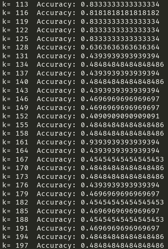
三、实验结论
由上图可知,随着 KNN 算法中 k 的值增大,算法的分类精度有显著的下降。
原因:较大的k值,相当于用较大的邻域中的训练实例进行预测,使模型简化。会减少噪音的影响,但是会使类别之间的界限变模糊,降低预测准确度;造成欠拟合。
感知机模型的构造
一、感知机原理
感知机是一个二类分类的线性分类器,是支持向量机和神经网络的基础。假设数据是线性可分的,目标是通过梯度下降法,极小化损失函数,最后找到一个分割超平面,可以将数据划分成两个类别。
- 模型流程图
import numpy as np

class Perceptron(object):
    '''
    eta:学习率
    n_iter:权重向量的训练次数
    w_:神经分叉权重向量
    error_:记录神经元判断出错次数
    '''

    def __init__(self, eta=0.01, n_iter=10):
        self.eta = eta
        self.n_iter = n_iter
        pass

    def fit(self, x, y):
        '''
        输入训练数据,训练神经元,x输入样本向量,y对应样本分类
        x:shape(n_samples,n_features)
        n_samples:样本量
        n_feature:神经元分叉数量
        例:x:[[1,2,3],[4,5,6]]
        n_samples:2
        n_feature:3
        y:[1,-1]
        '''
        '''
        初始化权重向量为0
        加一是因为将前面算法提到的w0,也就是步调函数阈值
        w_:权重向量
        error_:错误记录向量
        '''
        self.errors_ = []
        self.w_ = np.zeros(1 + x.shape[1])
        for _ in range(self.n_iter):
            errors = 0
            for xi, target in zip(x, y):
                '''
                zip(x,y):[[1,2,3,1],[4,5,6,-1]]
                '''
                update = (self.eta) * (target - self.predict(xi))
                self.w_[1:] += update * xi
                self.w_[0] += update
                '''
                ▽w(n) = update * x[n]
                '''
                errors += int(update != 0.0)
                self.errors_.append(errors)
                pass
            pass

    def net_input(self, x):
        '''
        z = w0 * 1 + w1 * x1 +... +wn * xn
        '''
        z = np.dot(x, self.w_[1:]) + self.w_[0]
        return z
        pass

    def predict(self, x):
        return np.where(self.net_input(x) >= 0.0, 1, -1)
        pass
import matplotlib.pyplot as plt
import matplotlib as mat
import pandas as pd
import numpy as np
df = pd.read_csv("https://archive.ics.uci.edu/ml/machine-learning-databases/iris/iris.data", header=None)
# 输出最后20行的数据,并观察数据结构 萼片长度(sepal length),萼片宽度(),
# 花瓣长度(petal length),花瓣宽度,种类
print(df.tail(n=20))
print(df.shape)
# 0到100行,第5列
y = df.iloc[0:100, 4].values
# 将target值转数字化 Iris-setosa为-1,否则值为1
y = np.where(y == "Iris-setosa", -1, 1)
# 取出0到100行,第1,第三列的值
x = df.iloc[0:100, [0, 2]].values
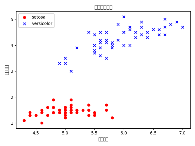
""" 鸢尾花散点图 """
# scatter绘制点图
plt.scatter(x[0:50, 0], x[0:50, 1], color="red", marker="o", label="setosa")
plt.scatter(x[50:100, 0], x[50:100, 1], color="blue", marker="x", label="versicolor")
# 防止中文乱码 下面分别是windows系统,mac系统解决中文乱码方案
# zhfont1 = mat.font_manager.FontProperties(fname='C:\Windows\Fonts\simsun.ttc')
# zhfont1 = mat.font_manager.FontProperties(fname='/System/Library/Fonts/PingFang.ttc')
plt.title("鸢尾花散点图")
plt.xlabel(u"萼片宽度")
plt.ylabel(u"花瓣宽度")
plt.legend(loc="upper left")
plt.show()
import matplotlib.pyplot as plt
import matplotlib as mat
import pandas as pd
import numpy as np

"""
    训练模型并且记录错误次数,观察错误次数的变化
"""
print(__doc__)
# 加载鸢尾花数据
df = pd.read_csv("https://archive.ics.uci.edu/ml/machine-learning-databases/iris/iris.data", header=None)

# 数据真实值
y = df.iloc[0:100, 4].values
y = np.where(y == "Iris-setosa", -1, 1)
x = df.iloc[0:100, [1, 3]].values
"""
    误差数折线图
    @:param eta: 0.1 学习速率
    @:param n_iter:0.1 迭代次数
"""
ppn = Perceptron(eta=0.1, n_iter=10)
ppn.fit(x, y)
# plot绘制折线图
plt.plot(range(1, len(ppn.errors_) + 1), ppn.errors_, marker="o")
# 防止中文乱码
# zhfont1 = mat.font_manager.FontProperties(fname='C:\Windows\Fonts\simsun.ttc')
plt.xlabel("迭代次数(n_iter)")
plt.ylabel("错误分类次数(error_number)")
plt.show()

import pandas as pd
import matplotlib as mat

from matplotlib.colors import ListedColormap
import numpy as np
import matplotlib.pyplot as plt


def plot_decision_regions(x, y, classifier, resolution=0.2):
    """
    二维数据集决策边界可视化
    :parameter
    -----------------------------
    :param self: 将鸢尾花花萼长度、花瓣长度进行可视化及分类
    :param x: list 被分类的样本
    :param y: list 样本对应的真实分类
    :param classifier: method  分类器:感知器
    :param resolution:
    :return:
    -----------------------------
    """
    markers = ('s', 'x', 'o', '^', 'v')
    colors = ('red', 'blue', 'lightgreen', 'gray', 'cyan')
    # y去重之后的种类
    listedColormap = ListedColormap(colors[:len(np.unique(y))])

    # 花萼长度最小值-1,最大值+1
    x1_min, x1_max = x[:, 0].min() - 1, x[:, 0].max() + 1
    # 花瓣长度最小值-1,最大值+1
    x2_min, x2_max = x[:, 1].min() - 1, x[:, 1].max() + 1

    # 将最大值,最小值向量生成二维数组xx1,xx2
    # np.arange(x1_min, x1_max, resolution)  最小值最大值中间,步长为resolution
    new_x1 = np.arange(x1_min, x1_max, resolution)
    new_x2 = np.arange(x2_min, x2_max, resolution)
    xx1, xx2 = np.meshgrid(new_x1, new_x2)

    # 预测值
    # z = classifier.predict([xx1, xx2])
    z = classifier.predict(np.array([xx1.ravel(), xx2.ravel()]).T)
    z = z.reshape(xx1.shape)
    plt.contourf(xx1, xx2, z, alpha=0.4)
    plt.xlim(xx1.min(), xx1.max())
    plt.ylim(xx2.min(), xx2.max())

    for idx, c1 in enumerate(np.unique(y)):
        plt.scatter(x=x[y == c1, 0], y=x[y == c1, 1], alpha=0.8, c=listedColormap(idx), marker=markers[idx], label=c1)


df = pd.read_csv("https://archive.ics.uci.edu/ml/machine-learning-databases/iris/iris.data", header=None)

# 0到100行,第5列
y = df.iloc[0:100, 4].values
# 将target值转数字化 Iris-setosa为-1,否则值为1,相当于激活函数-在此处表现为分段函数
y = np.where(y == "Iris-setosa", -1, 1)
# 取出0到100行,第1,第三列的值
x = df.iloc[0:100, [1, 3]].values
ppn = Perceptron(eta=0.1, n_iter=10)
ppn.fit(x, y)
plot_decision_regions(x, y, classifier=ppn)
# 防止中文乱码
# zhfont1 = mat.font_manager.FontProperties(fname='C:\Windows\Fonts\simsun.ttc')
plt.title("鸢尾花花瓣、花萼边界分割")
plt.xlabel("萼片宽度 [cm]")
plt.ylabel("花瓣宽度 [cm]")

# plt.legend(loc="uper left")
plt.show()
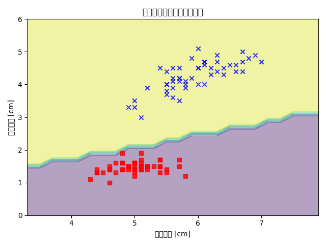
二、结论
使用 Iris 数据集的前 100 个记录,根据花萼宽度(第 2 列)、花瓣宽度(第 4 列)这两个特征对花进行分类,显示结果并分析能否正确分类?为什么?
根据第二列和第四列的属性值和对应的标签可视化如下,可以看到数据在二维平面上是线性可分的,因此感知机是完全可以正确分类的。

 浙公网安备 33010602011771号