作业三:使用minibatch的方式进行梯度下降
1、使用minibatch方式进行梯度下降
代码
import numpy as np
import matplotlib.pyplot as plt
from pathlib import Path
import random
x_data_name = "TemperatureControlXData.dat"
y_data_name = "TemperatureControlYData.dat"
class CData(object):
def __init__(self, loss, w, b, epoch, iteration):
self.loss = loss
self.w = w
self.b = b
self.epoch = epoch
self.iteration = iteration
def ReadData():
Xfile = Path(x_data_name)
Yfile = Path(y_data_name)
if Xfile.exists() & Yfile.exists():
X = np.load(Xfile)
Y = np.load(Yfile)
return X.reshape(1, -1), Y.reshape(1, -1)
else:
return None, None
def ForwardCalculationBatch(W, B, batch_x):
Z = np.dot(W, batch_x) + B
return Z
def BackPropagationBatch(batch_x, batch_y, batch_z):
m = batch_x.shape[1]
dZ = batch_z - batch_y
dB = dZ.sum(axis=1, keepdims=True) / m
dW = np.dot(dZ, batch_x.T) / m
return dW, dB
def UpdateWeights(w, b, dW, dB, eta):
w = w - eta * dW
b = b - eta * dB
return w, b
def InitialWeights(num_input, num_output, flag):
if flag == 0:
# zero
W = np.zeros((num_output, num_input))
elif flag == 1:
# normalize
W = np.random.normal(size=(num_output, num_input))
elif flag == 2:
# xavier
W = np.random.uniform(
-np.sqrt(6 / (num_input + num_output)),
np.sqrt(6 / (num_input + num_output)),
size=(num_output, num_input))
B = np.zeros((num_output, 1))
return W, B
def ShowResult(X, Y, w, b, iteration):
# draw sample data
plt.plot(X, Y, "b.")
# draw predication data
PX = np.linspace(0, 1, 10)
PZ = w * PX + b
plt.plot(PX, PZ, "r")
plt.title("Air Conditioner Power")
plt.xlabel("Number of Servers(K)")
plt.ylabel("Power of Air Conditioner(KW)")
plt.show()
print("iteration=", iteration)
print("w=%f,b=%f" % (w, b))
def CheckLoss(W, B, X, Y):
m = X.shape[1]
Z = np.dot(W, X) + B
LOSS = (Z - Y) ** 2
loss = LOSS.sum() / m / 2
return loss
def RandomSample(X,Y,batchsize):
batch_x = np.zeros((1,batchsize))
batch_y = np.zeros((1,batchsize))
for i in range(batchsize):
rvalue=random.randint(0,X.shape[1]-1)
batch_x[0,i] = X[0,rvalue]
X = np.delete(X,i,axis=1)
batch_y[0,i] = Y[0,rvalue]
Y = np.delete(Y,i,axis=1)
return batch_x, batch_y
# 从X和Y中随机选取数据
def GetMinimalLossData(dict_loss):
key = sorted(dict_loss.keys())[0]
w = dict_loss[key].w
b = dict_loss[key].b
return w, b, dict_loss[key]
def ShowLossHistory(dict_loss, method):
loss = []
for key in dict_loss:
loss.append(key)
# plt.plot(loss)
plt.plot(loss[30:800])
plt.title(method)
plt.xlabel("epoch")
plt.ylabel("loss")
plt.show()
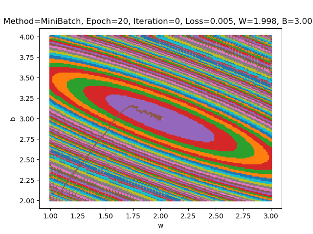
def loss_2d(x, y, n, dict_loss, method, cdata):
result_w = cdata.w[0, 0]
result_b = cdata.b[0, 0]
# show contour of loss
s = 150
W = np.linspace(result_w - 1, result_w + 1, s)
B = np.linspace(result_b - 1, result_b + 1, s)
LOSS = np.zeros((s, s))
for i in range(len(W)):
for j in range(len(B)):
w = W[i]
b = B[j]
a = w * x + b
loss = CheckLoss(w, b, x, y)
LOSS[i, j] = np.round(loss, 2)
# end for j
# end for i
print("please wait for 20 seconds...")
while (True):
X = []
Y = []
is_first = True
loss = 0
for i in range(len(W)):
for j in range(len(B)):
if LOSS[i, j] != 0:
if is_first:
loss = LOSS[i, j]
X.append(W[i])
Y.append(B[j])
LOSS[i, j] = 0
is_first = False
elif LOSS[i, j] == loss:
X.append(W[i])
Y.append(B[j])
LOSS[i, j] = 0
# end if
# end if
# end for j
# end for i
if is_first == True:
break
plt.plot(X, Y, '.')
# end while
# show w,b trace
w_history = []
b_history = []
for key in dict_loss:
w = dict_loss[key].w[0, 0]
b = dict_loss[key].b[0, 0]
if w < result_w - 1 or result_b - 1 < 2:
continue
if key == cdata.loss:
break
# end if
w_history.append(w)
b_history.append(b)
# end for
plt.plot(w_history, b_history)
plt.xlabel("w")
plt.ylabel("b")
title = str.format("Method={0}, Epoch={1}, Iteration={2}, Loss={3:.3f}, W={4:.3f}, B={5:.3f}", method, cdata.epoch,
cdata.iteration, cdata.loss, cdata.w[0, 0], cdata.b[0, 0])
plt.title(title)
plt.show()
def InitializeHyperParameters(method):
if method == "SGD":
eta = 0.1
max_epoch = 50
batch_size = 1
elif method == "MiniBatch":
eta = 0.1
max_epoch = 50
batch_size = 5
elif method == "FullBatch":
eta = 0.5
max_epoch = 1000
batch_size = 200
return eta, max_epoch, batch_size
if __name__ == '__main__':
# 修改method分别为下面三个参数,运行程序,对比不同的运行结果
# SGD, MiniBatch, FullBatch
method = "MiniBatch"
eta, max_epoch, batch_size = InitializeHyperParameters(method)
W, B = InitialWeights(1, 1, 0)
# calculate loss to decide the stop condition
loss = 5
dict_loss = {}
# read data
X, Y = ReadData()
# count of samples
num_example = X.shape[1]
num_feature = X.shape[0]
# if num_example=200, batch_size=10, then iteration=200/10=20
max_iteration = (int)(num_example / batch_size)
for epoch in range(max_epoch):
# 设置迭代次数
print("epoch=%d" % epoch)
for iteration in range(max_iteration):
# 根据batch_size确定循环次数
# get x and y value for one sample
batch_x, batch_y = RandomSample(X, Y, batch_size)
# get z from x,y
batch_z = ForwardCalculationBatch(W, B, batch_x)
# calculate gradient of w and b
dW, dB = BackPropagationBatch(batch_x, batch_y, batch_z)
# update w,b
W, B = UpdateWeights(W, B, dW, dB, eta)
# calculate loss for this batch
loss = CheckLoss(W, B, X, Y)
print(epoch, iteration, loss, W, B)
prev_loss = loss
dict_loss[loss] = CData(loss, W, B, epoch, iteration)
# end for
# end for
ShowLossHistory(dict_loss, method)
w, b, cdata = GetMinimalLossData(dict_loss)
print(cdata.w, cdata.b)
print("epoch=%d, iteration=%d, loss=%f" % (cdata.epoch, cdata.iteration, cdata.loss))
# ShowResult(X, Y, W, B, epoch)
print(w, b)
x = 346 / 1000
result = ForwardCalculationBatch(w, b, x)
print(result)
loss_2d(X, Y, 200, dict_loss, method, cdata)
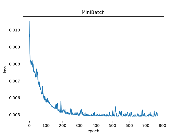
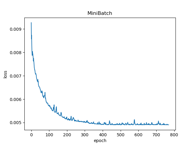
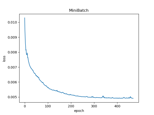
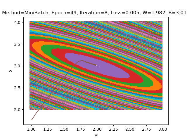
在batch_size不同的情况下进行结果分析
- batch_size=5
![]()
![]()
- batch_size=10
![]()
![]()
- batch_size=20
![]()
![]()
比较和思考
- 在batch_size比较小的时候,当训练值比较接近真实值的时候,s和b的波动会比较大;反之,当训练值比较接近真实值的时候,曲线变得更加平滑,样本的噪声变低。在训练速度上,两者并没有显著差异。这可能是由于样本总量比较小导致的。当样本数量比较大的时候,batch_size越大,训练的速度就越慢。
2、问题回答
1、为什么图像是椭圆而不是圆?
- 答:由于w和b的权重并不相同。如果我们想要得到一个圆,需要z对w和b的偏导数对于任意的x相同,也就是说这需要一个极其特殊的数据集使得对于数据集中的每一个元素(x,y),计算得到的z对w和b的偏导数相同。
2、为什么图像中心是一个区域而不是一个点?
- 答:由代码可知,损失函数图像中每一个颜色的色块代表损失函数在一个值域内的x(w,b)。在中心的那一部分,随着w和b的波动,损失函数的波动非常小,仍然在这一个值域内。


 浙公网安备 33010602011771号