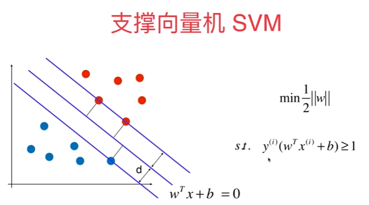
第11章支撑向量机 SVM

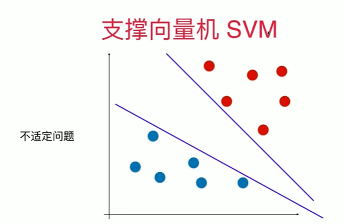
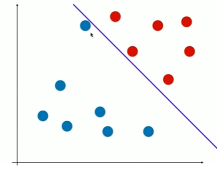
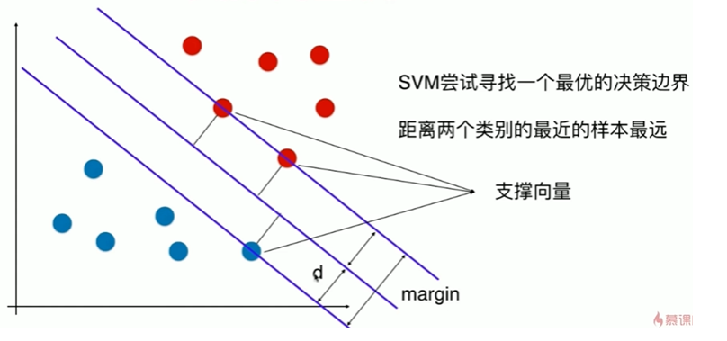
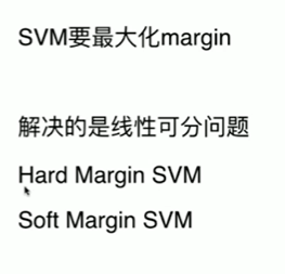
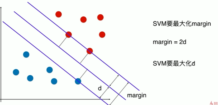
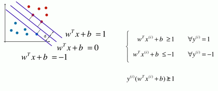
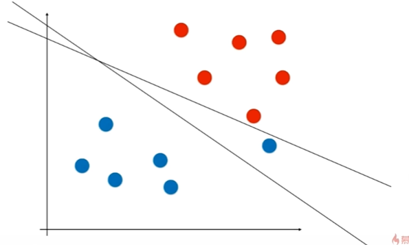
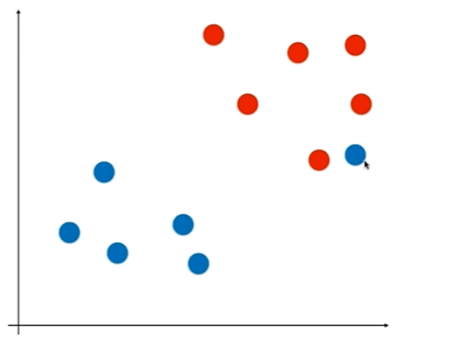
11-1 什么是支持向量机

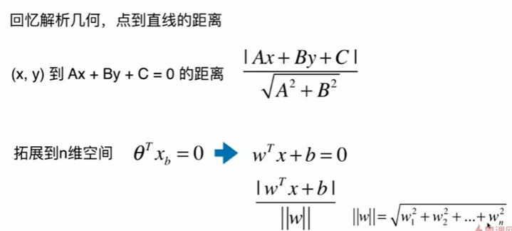
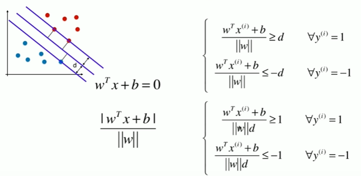
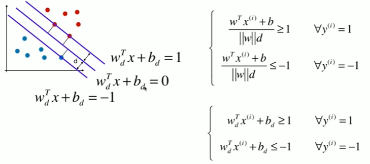
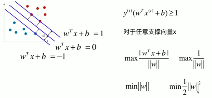
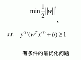
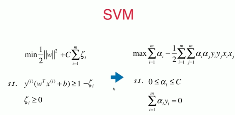
11-2 支持向量机的效用函数推导

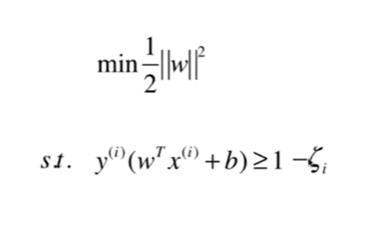
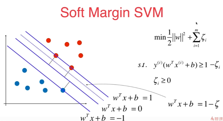
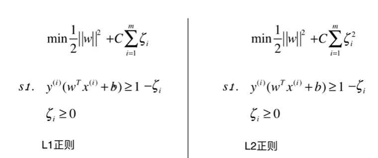
11-3 Soft Margin和SVM的正则化

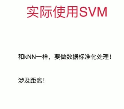
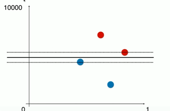
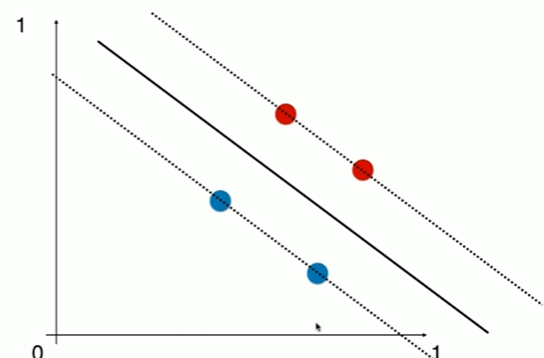
11-4 scikit-learn中的SVM

Notbook 示例

Notbook 源码

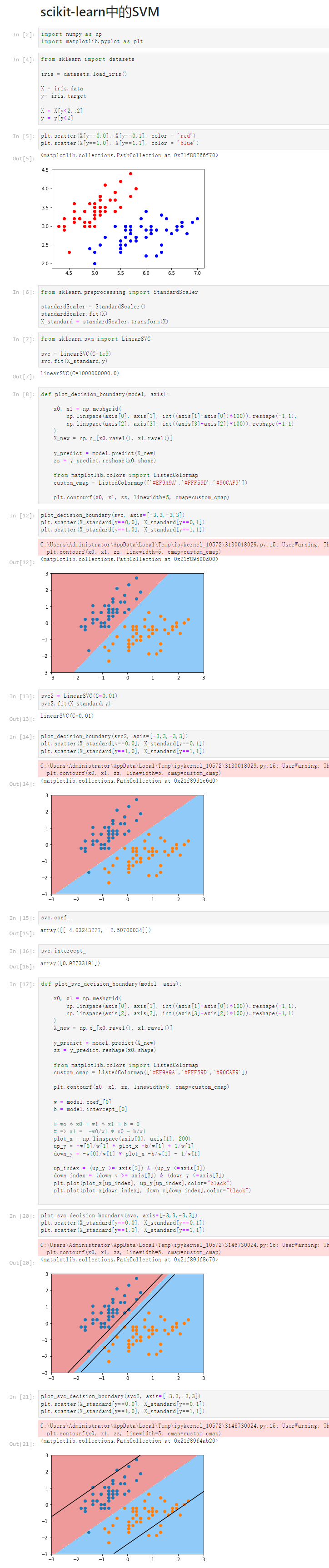
  1 scikit-learn中的SVM
  2 [2]
  3 import numpy as np
  4 import matplotlib.pyplot as plt
  5 [4]
  6 from sklearn import datasets
  7 
  8 iris = datasets.load_iris()
  9 
 10 X = iris.data
 11 y= iris.target
 12 
 13 X = X[y<2,:2]
 14 y = y[y<2]
 15 [5]
 16 plt.scatter(X[y==0,0], X[y==0,1], color = 'red')
 17 plt.scatter(X[y==1,0], X[y==1,1], color = 'blue')
 18 <matplotlib.collections.PathCollection at 0x21f88266f70>
 19 
 20 [6]
 21 from sklearn.preprocessing import StandardScaler
 22 
 23 standardScaler = StandardScaler()
 24 standardScaler.fit(X)
 25 X_standard = standardScaler.transform(X)
 26 [7]
 27 from sklearn.svm import LinearSVC
 28 
 29 svc = LinearSVC(C=1e9)
 30 svc.fit(X_standard,y)
 31 LinearSVC(C=1000000000.0)
 32 [8]
 33 def plot_decision_boundary(model, axis):
 34 
 35     x0, x1 = np.meshgrid(
 36         np.linspace(axis[0], axis[1], int((axis[1]-axis[0])*100)).reshape(-1,1),
 37         np.linspace(axis[2], axis[3], int((axis[3]-axis[2])*100)).reshape(-1,1)
 38     )
 39     X_new = np.c_[x0.ravel(), x1.ravel()]
 40     
 41     y_predict = model.predict(X_new)
 42     zz = y_predict.reshape(x0.shape)
 43 
 44     from matplotlib.colors import ListedColormap
 45     custom_cmap = ListedColormap(['#EF9A9A','#FFF59D','#90CAF9'])
 46     
 47     plt.contourf(x0, x1, zz, linewidth=5, cmap=custom_cmap)
 48 [12]
 49 plot_decision_boundary(svc, axis=[-3,3,-3,3])
 50 plt.scatter(X_standard[y==0,0], X_standard[y==0,1])
 51 plt.scatter(X_standard[y==1,0], X_standard[y==1,1])
 52 C:\Users\Administrator\AppData\Local\Temp\ipykernel_10572\3130018029.py:15: UserWarning: The following kwargs were not used by contour: 'linewidth'
 53   plt.contourf(x0, x1, zz, linewidth=5, cmap=custom_cmap)
 54 
 55 <matplotlib.collections.PathCollection at 0x21f89d00d00>
 56 
 57 [13]
 58 svc2 = LinearSVC(C=0.01)
 59 svc2.fit(X_standard,y)
 60 LinearSVC(C=0.01)
 61 [14]
 62 plot_decision_boundary(svc2, axis=[-3,3,-3,3])
 63 plt.scatter(X_standard[y==0,0], X_standard[y==0,1])
 64 plt.scatter(X_standard[y==1,0], X_standard[y==1,1])
 65 C:\Users\Administrator\AppData\Local\Temp\ipykernel_10572\3130018029.py:15: UserWarning: The following kwargs were not used by contour: 'linewidth'
 66   plt.contourf(x0, x1, zz, linewidth=5, cmap=custom_cmap)
 67 
 68 <matplotlib.collections.PathCollection at 0x21f89d1c6d0>
 69 
 70 [15]
 71 svc.coef_
 72 array([[ 4.03243277, -2.50700034]])
 73 [16]
 74 svc.intercept_
 75 array([0.92733191])
 76 [17]
 77 def plot_svc_decision_boundary(model, axis):
 78 
 79     x0, x1 = np.meshgrid(
 80         np.linspace(axis[0], axis[1], int((axis[1]-axis[0])*100)).reshape(-1,1),
 81         np.linspace(axis[2], axis[3], int((axis[3]-axis[2])*100)).reshape(-1,1)
 82     )
 83     X_new = np.c_[x0.ravel(), x1.ravel()]
 84     
 85     y_predict = model.predict(X_new)
 86     zz = y_predict.reshape(x0.shape)
 87 
 88     from matplotlib.colors import ListedColormap
 89     custom_cmap = ListedColormap(['#EF9A9A','#FFF59D','#90CAF9'])
 90     
 91     plt.contourf(x0, x1, zz, linewidth=5, cmap=custom_cmap)
 92     
 93     w = model.coef_[0]
 94     b = model.intercept_[0]
 95     
 96     # wo * x0 + w1 * x1 + b = 0
 97     # => x1 =  -w0/w1 * x0 - b/w1
 98     plot_x = np.linspace(axis[0], axis[1], 200)
 99     up_y = -w[0]/w[1] * plot_x -b/w[1] + 1/w[1]
100     down_y = -w[0]/w[1] * plot_x -b/w[1] - 1/w[1]
101         
102     up_index = (up_y >= axis[2]) & (up_y <=axis[3])    
103     down_index = (down_y >= axis[2]) & (down_y <=axis[3]) 
104     plt.plot(plot_x[up_index], up_y[up_index],color="black")
105     plt.plot(plot_x[down_index], down_y[down_index],color="black")
106     
107 [20]
108 plot_svc_decision_boundary(svc, axis=[-3,3,-3,3])
109 plt.scatter(X_standard[y==0,0], X_standard[y==0,1])
110 plt.scatter(X_standard[y==1,0], X_standard[y==1,1])
111 C:\Users\Administrator\AppData\Local\Temp\ipykernel_10572\3146730024.py:15: UserWarning: The following kwargs were not used by contour: 'linewidth'
112   plt.contourf(x0, x1, zz, linewidth=5, cmap=custom_cmap)
113 
114 <matplotlib.collections.PathCollection at 0x21f89df8c70>
115 
116 [21]
117 plot_svc_decision_boundary(svc2, axis=[-3,3,-3,3])
118 plt.scatter(X_standard[y==0,0], X_standard[y==0,1])
119 plt.scatter(X_standard[y==1,0], X_standard[y==1,1])
120 C:\Users\Administrator\AppData\Local\Temp\ipykernel_10572\3146730024.py:15: UserWarning: The following kwargs were not used by contour: 'linewidth'
121   plt.contourf(x0, x1, zz, linewidth=5, cmap=custom_cmap)
122 
123 <matplotlib.collections.PathCollection at 0x21f89f4ab20>

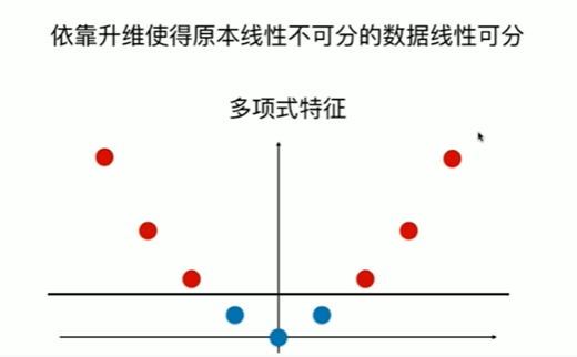
11-5 SVM中使用多项式特征

Notbook 示例

Notbook 源码

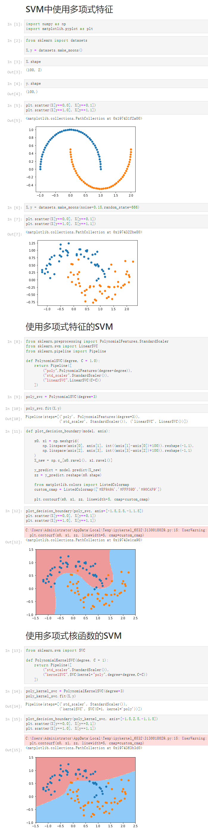
 1 SVM中使用多项式特征
 2 [1]
 3 import numpy as np
 4 import matplotlib.pyplot as plt
 5 [2]
 6 from sklearn import datasets
 7 
 8 X,y = datasets.make_moons()
 9 [3]
10 X.shape
11 (100, 2)
12 [4]
13 y.shape
14 (100,)
15 [5]
16 plt.scatter(X[y==0,0], X[y==0,1])
17 plt.scatter(X[y==1,0], X[y==1,1])
18 <matplotlib.collections.PathCollection at 0x197431f2a00>
19 
20 [6]
21 X,y = datasets.make_moons(noise=0.15,random_state=666)
22 [7]
23 plt.scatter(X[y==0,0], X[y==0,1])
24 plt.scatter(X[y==1,0], X[y==1,1])
25 <matplotlib.collections.PathCollection at 0x1974322be80>
26 
27 使用多项式特征的SVM
28 [8]
29 from sklearn.preprocessing import PolynomialFeatures,StandardScaler
30 from sklearn.svm import LinearSVC
31 from sklearn.pipeline import Pipeline
32 
33 def PolynomialSVC(degree, C = 1.0):
34     return Pipeline([
35         ("poly",PolynomialFeatures(degree=degree)),
36         ("std_scaler",StandardScaler()),
37         ("linearSVC",LinearSVC(C=C))
38     ])
39 [9]
40 poly_svc = PolynomialSVC(degree=3)
41 [10]
42 poly_svc.fit(X,y)
43 Pipeline(steps=[('poly', PolynomialFeatures(degree=3)),
44                 ('std_scaler', StandardScaler()), ('linearSVC', LinearSVC())])
45 [11]
46 def plot_decision_boundary(model, axis):
47 
48     x0, x1 = np.meshgrid(
49         np.linspace(axis[0], axis[1], int((axis[1]-axis[0])*100)).reshape(-1,1),
50         np.linspace(axis[2], axis[3], int((axis[3]-axis[2])*100)).reshape(-1,1)
51     )
52     X_new = np.c_[x0.ravel(), x1.ravel()]
53     
54     y_predict = model.predict(X_new)
55     zz = y_predict.reshape(x0.shape)
56 
57     from matplotlib.colors import ListedColormap
58     custom_cmap = ListedColormap(['#EF9A9A','#FFF59D','#90CAF9'])
59     
60     plt.contourf(x0, x1, zz, linewidth=5, cmap=custom_cmap)
61 [12]
62 plot_decision_boundary(poly_svc, axis=[-1.5,2.5,-1,1.5])
63 plt.scatter(X[y==0,0], X[y==0,1])
64 plt.scatter(X[y==1,0], X[y==1,1])
65 C:\Users\Administrator\AppData\Local\Temp\ipykernel_6532\3130018029.py:15: UserWarning: The following kwargs were not used by contour: 'linewidth'
66   plt.contourf(x0, x1, zz, linewidth=5, cmap=custom_cmap)
67 
68 <matplotlib.collections.PathCollection at 0x19743e1ca90>
69 
70 使用多项式核函数的SVM
71 [13]
72 from sklearn.svm import SVC
73 
74 def PolynomialKernelSVC(degree, C = 1):
75     return Pipeline([
76         ("std_scaler",StandardScaler()),
77         ("kernelSVC",SVC(kernel="poly",degree=degree,C=C))
78     ])
79 [14]
80 poly_kernel_svc = PolynomialKernelSVC(degree=3)
81 poly_kernel_svc.fit(X,y)
82 Pipeline(steps=[('std_scaler', StandardScaler()),
83                 ('kernelSVC', SVC(C=1, kernel='poly'))])
84 [15]
85 plot_decision_boundary(poly_kernel_svc, axis=[-1.5,2.5,-1,1.5])
86 plt.scatter(X[y==0,0], X[y==0,1])
87 plt.scatter(X[y==1,0], X[y==1,1])
88 C:\Users\Administrator\AppData\Local\Temp\ipykernel_6532\3130018029.py:15: UserWarning: The following kwargs were not used by contour: 'linewidth'
89   plt.contourf(x0, x1, zz, linewidth=5, cmap=custom_cmap)
90 
91 <matplotlib.collections.PathCollection at 0x1974363b3d0>

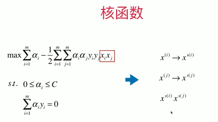
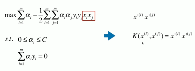
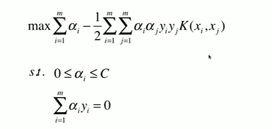
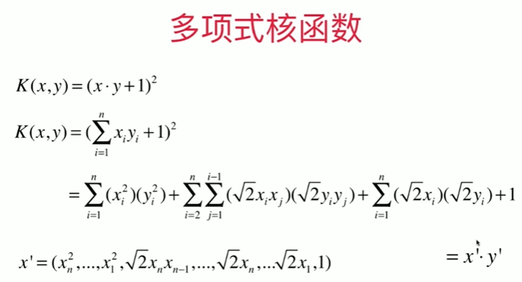
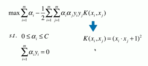
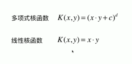
11-6 核函数

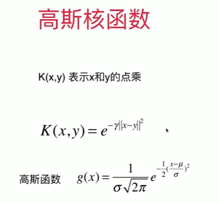
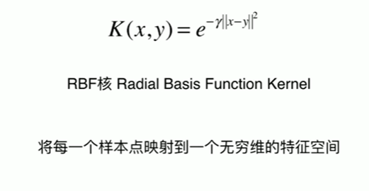
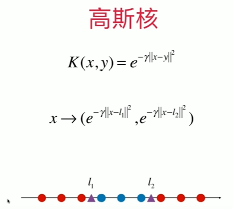
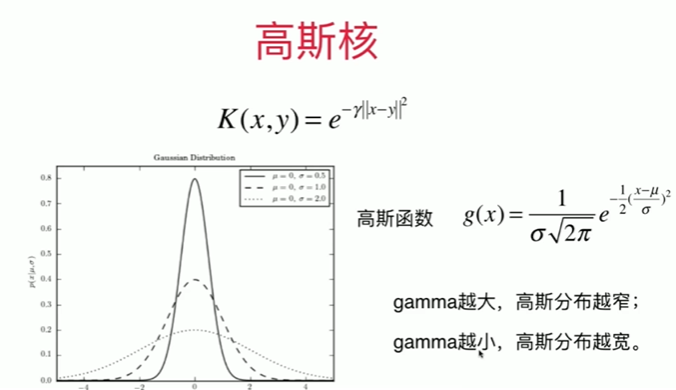
11-7 高斯核函数

Notbook 示例

Notbook 源码

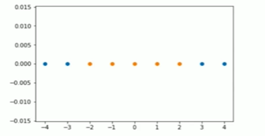
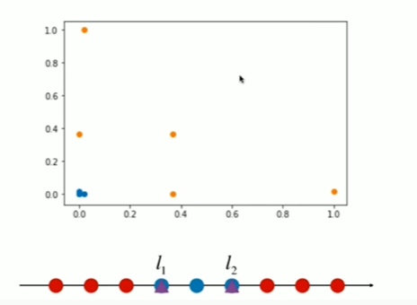
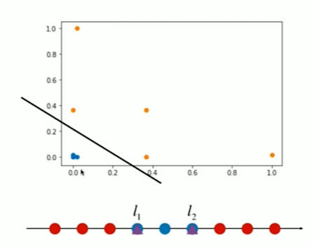
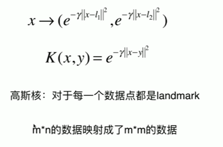
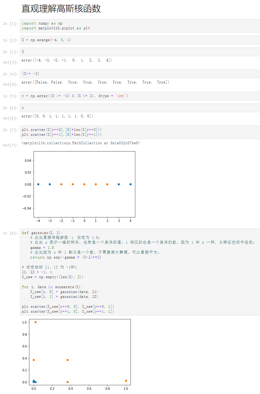
 1 直观理解高斯核函数
 2 [1]
 3 import numpy as np
 4 import matplotlib.pyplot as plt
 5 [2]
 6 X = np.arange(-4, 5, 1)
 7 [3]
 8 X
 9 array([-4, -3, -2, -1,  0,  1,  2,  3,  4])
10 [4]
11 (X>= -2)
12 array([False, False,  True,  True,  True,  True,  True,  True,  True])
13 [5]
14 y = np.array((X >= -2) & (X <= 2), dtype = 'int')
15 [6]
16 y
17 array([0, 0, 1, 1, 1, 1, 1, 0, 0])
18 [7]
19 plt.scatter(X[y==0],[0]*len(X[y==0]))
20 plt.scatter(X[y==1],[0]*len(X[y==1]))
21 <matplotlib.collections.PathCollection at 0x1e532c07be0>
22 
23 [8]
24 def gaussian(X, l):
25     # 此处直接将超参数 γ 设定为 1.0；
26     # 此处 x 表示一维的样本，也就是一个具体的值，l 相应的也是一个具体的数，因为 l 和 x 一样，从特征空间中选定；
27     gamma = 1.0
28     # 此处因为 x 和 l 都只是一个数，不需要再计算模，可以直接平方；
29     return np.exp(-gamma * (X-l)**2)
30 
31 # 设定地标 l1、l2 为 -1和1
32 l1, l2 = -1, 1
33 X_new = np.empty((len(X), 2))
34 
35 for i, data in enumerate(X):
36     X_new[i, 0] = gaussian(data, l1)
37     X_new[i, 1] = gaussian(data, l2)
38 
39 plt.scatter(X_new[y==0, 0], X_new[y==0, 1])
40 plt.scatter(X_new[y==1, 0], X_new[y==1, 1])

11-8 scikit-learn中的高斯核函数

Notbook 示例

Notbook 源码

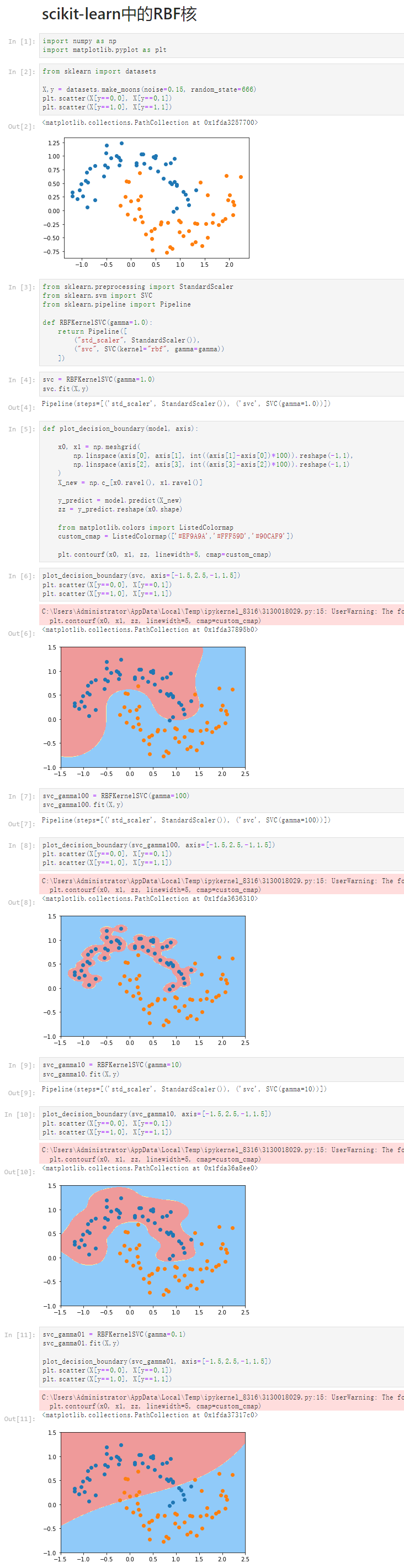
 1 scikit-learn中的RBF核
 2 [1]
 3 import numpy as np
 4 import matplotlib.pyplot as plt
 5 [2]
 6 from sklearn import datasets
 7 
 8 X,y = datasets.make_moons(noise=0.15, random_state=666)
 9 plt.scatter(X[y==0,0], X[y==0,1])
10 plt.scatter(X[y==1,0], X[y==1,1])
11 <matplotlib.collections.PathCollection at 0x1fda3257700>
12 
13 [3]
14 from sklearn.preprocessing import StandardScaler
15 from sklearn.svm import SVC
16 from sklearn.pipeline import Pipeline
17 
18 def RBFKernelSVC(gamma=1.0):
19     return Pipeline([
20         ("std_scaler", StandardScaler()),
21         ("svc", SVC(kernel="rbf", gamma=gamma))
22     ])
23 [4]
24 svc = RBFKernelSVC(gamma=1.0)
25 svc.fit(X,y)
26 Pipeline(steps=[('std_scaler', StandardScaler()), ('svc', SVC(gamma=1.0))])
27 [5]
28 def plot_decision_boundary(model, axis):
29 
30     x0, x1 = np.meshgrid(
31         np.linspace(axis[0], axis[1], int((axis[1]-axis[0])*100)).reshape(-1,1),
32         np.linspace(axis[2], axis[3], int((axis[3]-axis[2])*100)).reshape(-1,1)
33     )
34     X_new = np.c_[x0.ravel(), x1.ravel()]
35     
36     y_predict = model.predict(X_new)
37     zz = y_predict.reshape(x0.shape)
38 
39     from matplotlib.colors import ListedColormap
40     custom_cmap = ListedColormap(['#EF9A9A','#FFF59D','#90CAF9'])
41     
42     plt.contourf(x0, x1, zz, linewidth=5, cmap=custom_cmap)
43 [6]
44 plot_decision_boundary(svc, axis=[-1.5,2.5,-1,1.5])
45 plt.scatter(X[y==0,0], X[y==0,1])
46 plt.scatter(X[y==1,0], X[y==1,1])
47 C:\Users\Administrator\AppData\Local\Temp\ipykernel_8316\3130018029.py:15: UserWarning: The following kwargs were not used by contour: 'linewidth'
48   plt.contourf(x0, x1, zz, linewidth=5, cmap=custom_cmap)
49 
50 <matplotlib.collections.PathCollection at 0x1fda37895b0>
51 
52 [7]
53 svc_gamma100 = RBFKernelSVC(gamma=100)
54 svc_gamma100.fit(X,y)
55 Pipeline(steps=[('std_scaler', StandardScaler()), ('svc', SVC(gamma=100))])
56 [8]
57 plot_decision_boundary(svc_gamma100, axis=[-1.5,2.5,-1,1.5])
58 plt.scatter(X[y==0,0], X[y==0,1])
59 plt.scatter(X[y==1,0], X[y==1,1])
60 C:\Users\Administrator\AppData\Local\Temp\ipykernel_8316\3130018029.py:15: UserWarning: The following kwargs were not used by contour: 'linewidth'
61   plt.contourf(x0, x1, zz, linewidth=5, cmap=custom_cmap)
62 
63 <matplotlib.collections.PathCollection at 0x1fda3636310>
64 
65 [9]
66 svc_gamma10 = RBFKernelSVC(gamma=10)
67 svc_gamma10.fit(X,y)
68 Pipeline(steps=[('std_scaler', StandardScaler()), ('svc', SVC(gamma=10))])
69 [10]
70 plot_decision_boundary(svc_gamma10, axis=[-1.5,2.5,-1,1.5])
71 plt.scatter(X[y==0,0], X[y==0,1])
72 plt.scatter(X[y==1,0], X[y==1,1])
73 C:\Users\Administrator\AppData\Local\Temp\ipykernel_8316\3130018029.py:15: UserWarning: The following kwargs were not used by contour: 'linewidth'
74   plt.contourf(x0, x1, zz, linewidth=5, cmap=custom_cmap)
75 
76 <matplotlib.collections.PathCollection at 0x1fda36a8ee0>
77 
78 [11]
79 svc_gamma01 = RBFKernelSVC(gamma=0.1)
80 svc_gamma01.fit(X,y)
81 
82 plot_decision_boundary(svc_gamma01, axis=[-1.5,2.5,-1,1.5])
83 plt.scatter(X[y==0,0], X[y==0,1])
84 plt.scatter(X[y==1,0], X[y==1,1])
85 C:\Users\Administrator\AppData\Local\Temp\ipykernel_8316\3130018029.py:15: UserWarning: The following kwargs were not used by contour: 'linewidth'
86   plt.contourf(x0, x1, zz, linewidth=5, cmap=custom_cmap)
87 
88 <matplotlib.collections.PathCollection at 0x1fda37317c0>

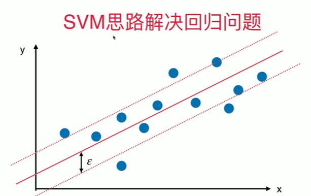
11-9 SVM思路解决回归问题

Notbook 示例

Notbook 源码

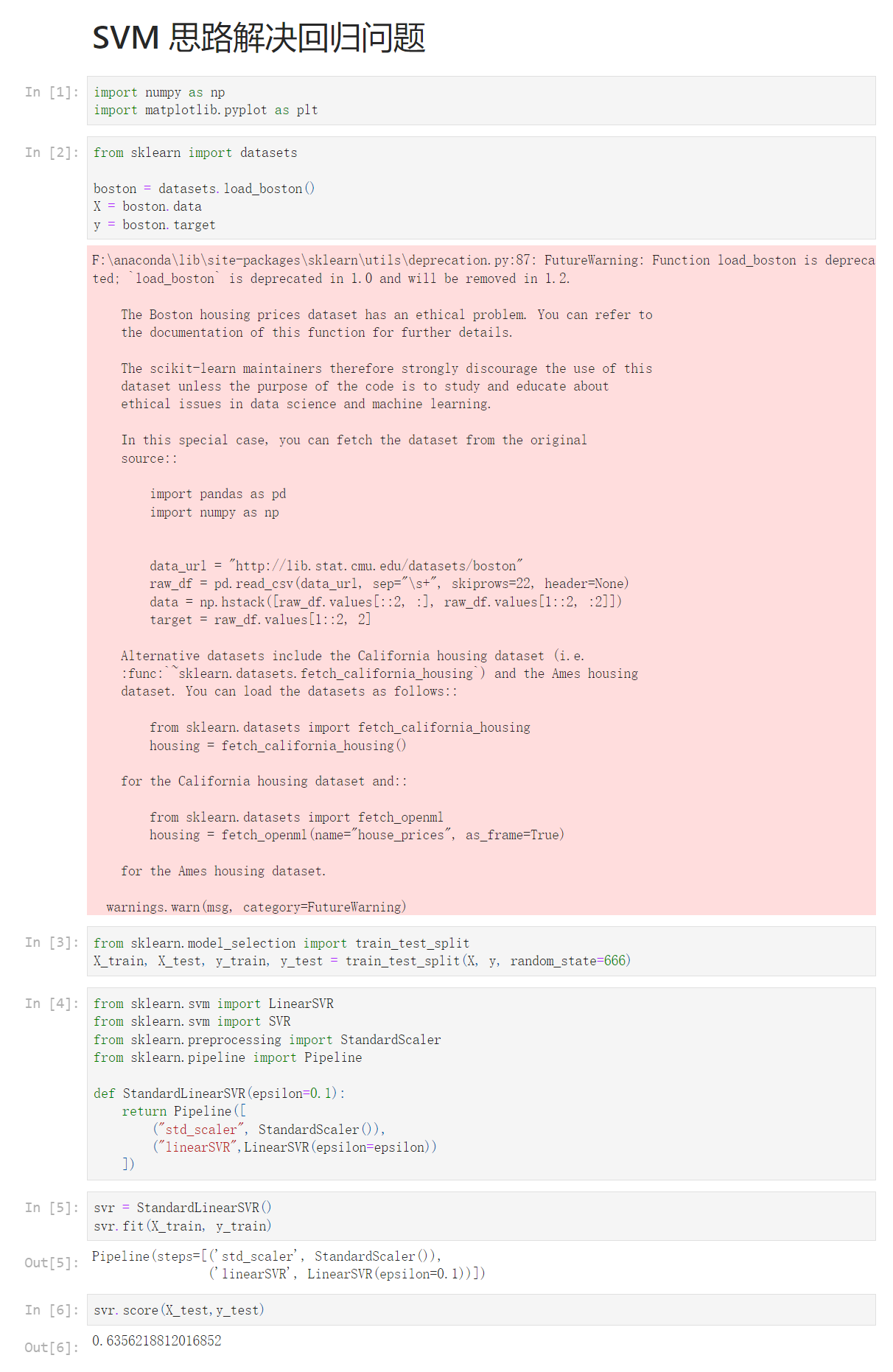
 1 SVM 思路解决回归问题
 2 [1]
 3 import numpy as np
 4 import matplotlib.pyplot as plt
 5 [2]
 6 from sklearn import datasets
 7 
 8 boston = datasets.load_boston()
 9 X = boston.data
10 y = boston.target
11 F:\anaconda\lib\site-packages\sklearn\utils\deprecation.py:87: FutureWarning: Function load_boston is deprecated; `load_boston` is deprecated in 1.0 and will be removed in 1.2.
12 
13     The Boston housing prices dataset has an ethical problem. You can refer to
14     the documentation of this function for further details.
15 
16     The scikit-learn maintainers therefore strongly discourage the use of this
17     dataset unless the purpose of the code is to study and educate about
18     ethical issues in data science and machine learning.
19 
20     In this special case, you can fetch the dataset from the original
21     source::
22 
23         import pandas as pd
24         import numpy as np
25 
26 
27         data_url = "http://lib.stat.cmu.edu/datasets/boston"
28         raw_df = pd.read_csv(data_url, sep="\s+", skiprows=22, header=None)
29         data = np.hstack([raw_df.values[::2, :], raw_df.values[1::2, :2]])
30         target = raw_df.values[1::2, 2]
31 
32     Alternative datasets include the California housing dataset (i.e.
33     :func:`~sklearn.datasets.fetch_california_housing`) and the Ames housing
34     dataset. You can load the datasets as follows::
35 
36         from sklearn.datasets import fetch_california_housing
37         housing = fetch_california_housing()
38 
39     for the California housing dataset and::
40 
41         from sklearn.datasets import fetch_openml
42         housing = fetch_openml(name="house_prices", as_frame=True)
43 
44     for the Ames housing dataset.
45     
46   warnings.warn(msg, category=FutureWarning)
47 
48 [3]
49 from sklearn.model_selection import train_test_split
50 X_train, X_test, y_train, y_test = train_test_split(X, y, random_state=666)
51 [4]
52 from sklearn.svm import LinearSVR
53 from sklearn.svm import SVR
54 from sklearn.preprocessing import StandardScaler
55 from sklearn.pipeline import Pipeline
56 
57 def StandardLinearSVR(epsilon=0.1):
58     return Pipeline([
59         ("std_scaler", StandardScaler()),
60         ("linearSVR",LinearSVR(epsilon=epsilon))
61     ])
62 [5]
63 svr = StandardLinearSVR()
64 svr.fit(X_train, y_train)
65 Pipeline(steps=[('std_scaler', StandardScaler()),
66                 ('linearSVR', LinearSVR(epsilon=0.1))])
67 [6]
68 svr.score(X_test,y_test)
69 0.6356218812016852

posted @ 2022-10-31 12:24 Cai-Gbro 阅读(69) 评论(0) 收藏举报

刷新页面返回顶部

Cai-Gbro

第11章 支撑向量机 SVM

11-1 什么是支持向量机

11-2 支持向量机的效用函数推导

11-3 Soft Margin和SVM的正则化

11-4 scikit-learn中的SVM

Notbook 示例

Notbook 源码

11-5 SVM中使用多项式特征

Notbook 示例

Notbook 源码

11-6 核函数

11-7 高斯核函数

Notbook 示例

Notbook 源码

11-8 scikit-learn中的高斯核函数

Notbook 示例

Notbook 源码

11-9 SVM思路解决回归问题

Notbook 示例

Notbook 源码

公告

第11章支撑向量机 SVM