


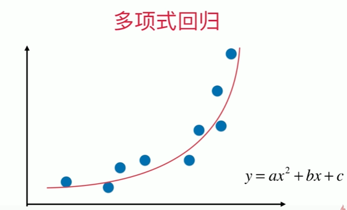
第8章上 多项式回归与模型泛化
8-1 什么是多项式回归
Notbook 示例
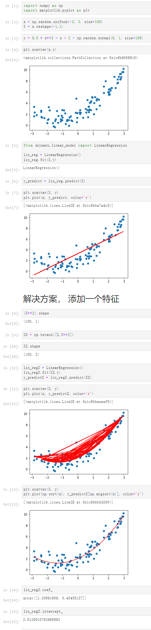
Notbook 源码
 1 [1]
 2 import numpy as np
 3 import matplotlib.pyplot as plt
 4 [2]
 5 x = np.random.uniform(-3, 3, size=100)
 6 X = x.reshape(-1,1)
 7 [3]
 8 y = 0.5 * x**2 + x + 2 + np.random.normal(0, 1, size=100)
 9 [4]
10 plt.scatter(x,y)
11 <matplotlib.collections.PathCollection at 0x1c6b9056910>
12
13 [5]
14 from sklearn.linear_model import LinearRegression
15
16 lin_reg = LinearRegression()
17 lin_reg.fit(X,y)
18 LinearRegression()
19 [6]
20 y_predict = lin_reg.predict(X)
21 [7]
22 plt.scatter(X, y)
23 plt.plot(x, y_predict, color='r')
24 [<matplotlib.lines.Line2D at 0x1c6bba7a4c0>]
25
26 解决方案, 添加一个特征
27 [8]
28 (X**2).shape
29 (100, 1)
30 [9]
31 X2 = np.hstack([X,X**2])
32 [10]
33 X2.shape
34 (100, 2)
35 [11]
36 lin_reg2 = LinearRegression()
37 lin_reg2.fit(X2,y)
38 y_predict2 = lin_reg2.predict(X2)
39 [12]
40 plt.scatter(X, y)
41 plt.plot(x, y_predict2, color='r')
42 [<matplotlib.lines.Line2D at 0x1c6bbaeaaf0>]
43
44 [13]
45 plt.scatter(X, y)
46 plt.plot(np.sort(x), y_predict2[np.argsort(x)], color='r')
47 [<matplotlib.lines.Line2D at 0x1c6bbb5d580>]
48
49 [14]
50 lin_reg2.coef_
51 array([1.20691609, 0.45458127])
52 [15]
53 lin_reg2.intercept_
54 2.0128010763968693
8-2 scikit-learn中的多项式回归于pipeline
Notbook 示例
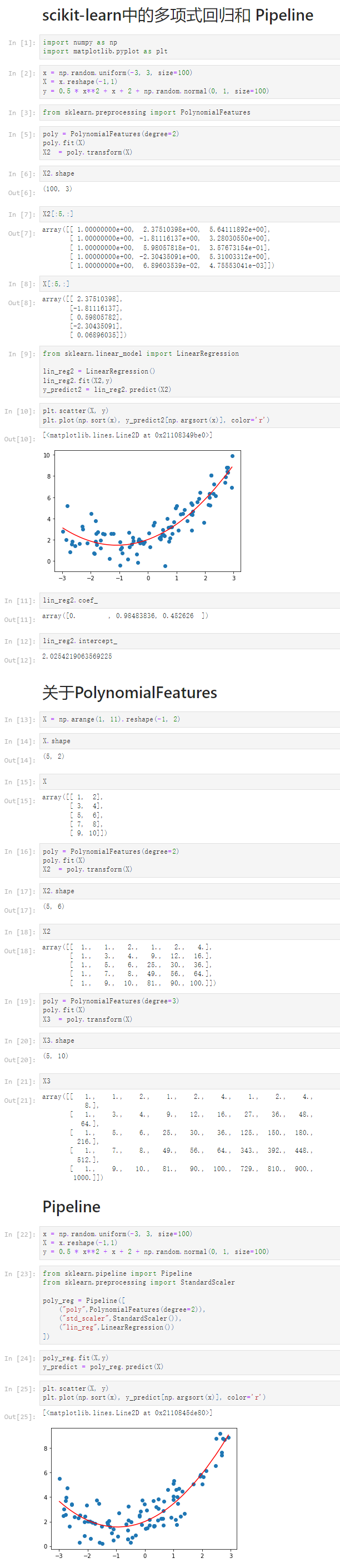
Notbook 源码
  1 scikit-learn中的多项式回归和 Pipeline
  2 [1]
  3 import numpy as np
  4 import matplotlib.pyplot as plt
  5 [2]
  6 x = np.random.uniform(-3, 3, size=100)
  7 X = x.reshape(-1,1)
  8 y = 0.5 * x**2 + x + 2 + np.random.normal(0, 1, size=100)
  9 [3]
 10 from sklearn.preprocessing import PolynomialFeatures
 11 [5]
 12 poly = PolynomialFeatures(degree=2)
 13 poly.fit(X)
 14 X2  = poly.transform(X)
 15 [6]
 16 X2.shape
 17 (100, 3)
 18 [7]
 19 X2[:5,:]
 20 array([[ 1.00000000e+00,  2.37510398e+00,  5.64111892e+00],
 21        [ 1.00000000e+00, -1.81116137e+00,  3.28030550e+00],
 22        [ 1.00000000e+00,  5.98057818e-01,  3.57673154e-01],
 23        [ 1.00000000e+00, -2.30435091e+00,  5.31003312e+00],
 24        [ 1.00000000e+00,  6.89603539e-02,  4.75553041e-03]])
 25 [8]
 26 X[:5,:]
 27 array([[ 2.37510398],
 28        [-1.81116137],
 29        [ 0.59805782],
 30        [-2.30435091],
 31        [ 0.06896035]])
 32 [9]
 33 from sklearn.linear_model import LinearRegression
 34
 35 lin_reg2 = LinearRegression()
 36 lin_reg2.fit(X2,y)
 37 y_predict2 = lin_reg2.predict(X2)
 38 [10]
 39 plt.scatter(X, y)
 40 plt.plot(np.sort(x), y_predict2[np.argsort(x)], color='r')
 41 [<matplotlib.lines.Line2D at 0x21108349be0>]
 42
 43 [11]
 44 lin_reg2.coef_
 45 array([0.        , 0.98483836, 0.452626  ])
 46 [12]
 47 lin_reg2.intercept_
 48 2.0254219063569225
 49 关于PolynomialFeatures
 50 [13]
 51 X = np.arange(1, 11).reshape(-1, 2)
 52 [14]
 53 X.shape
 54 (5, 2)
 55 [15]
 56 X
 57 array([[ 1,  2],
 58        [ 3,  4],
 59        [ 5,  6],
 60        [ 7,  8],
 61        [ 9, 10]])
 62 [16]
 63 poly = PolynomialFeatures(degree=2)
 64 poly.fit(X)
 65 X2  = poly.transform(X)
 66 [17]
 67 X2.shape
 68 (5, 6)
 69 [18]
 70 X2
 71 array([[  1.,   1.,   2.,   1.,   2.,   4.],
 72        [  1.,   3.,   4.,   9.,  12.,  16.],
 73        [  1.,   5.,   6.,  25.,  30.,  36.],
 74        [  1.,   7.,   8.,  49.,  56.,  64.],
 75        [  1.,   9.,  10.,  81.,  90., 100.]])
 76 [19]
 77 poly = PolynomialFeatures(degree=3)
 78 poly.fit(X)
 79 X3  = poly.transform(X)
 80 [20]
 81 X3.shape
 82 (5, 10)
 83 [21]
 84 X3
 85 array([[   1.,    1.,    2.,    1.,    2.,    4.,    1.,    2.,    4.,
 86            8.],
 87        [   1.,    3.,    4.,    9.,   12.,   16.,   27.,   36.,   48.,
 88           64.],
 89        [   1.,    5.,    6.,   25.,   30.,   36.,  125.,  150.,  180.,
 90          216.],
 91        [   1.,    7.,    8.,   49.,   56.,   64.,  343.,  392.,  448.,
 92          512.],
 93        [   1.,    9.,   10.,   81.,   90.,  100.,  729.,  810.,  900.,
 94         1000.]])
 95 Pipeline
 96 [22]
 97 x = np.random.uniform(-3, 3, size=100)
 98 X = x.reshape(-1,1)
 99 y = 0.5 * x**2 + x + 2 + np.random.normal(0, 1, size=100)
100 [23]
101 from sklearn.pipeline import Pipeline
102 from sklearn.preprocessing import StandardScaler
103
104 poly_reg = Pipeline([
105     ("poly",PolynomialFeatures(degree=2)),
106     ("std_scaler",StandardScaler()),
107     ("lin_reg",LinearRegression())
108 ])
109 [24]
110 poly_reg.fit(X,y)
111 y_predict = poly_reg.predict(X)
112 [25]
113 plt.scatter(X, y)
114 plt.plot(np.sort(x), y_predict[np.argsort(x)], color='r')
115 [<matplotlib.lines.Line2D at 0x2110845de80>]
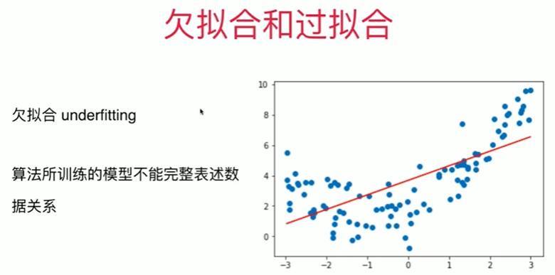
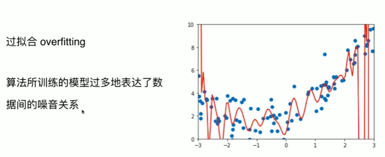
8-3 过拟合与欠拟合
Notbook 示例
Notbook 源码
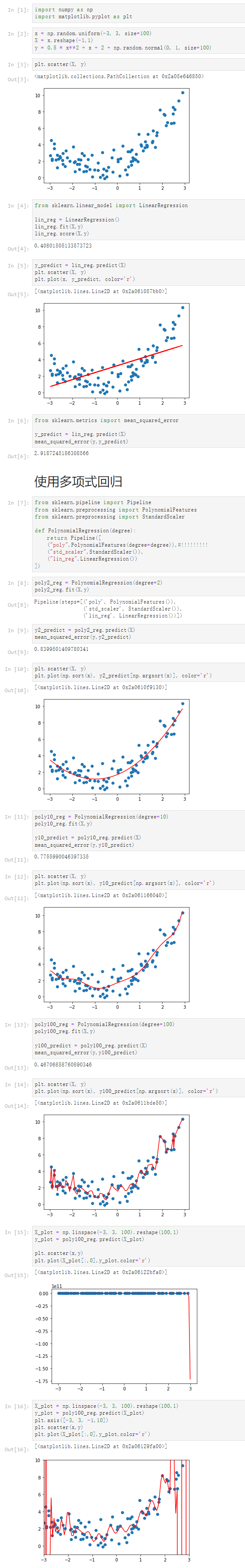
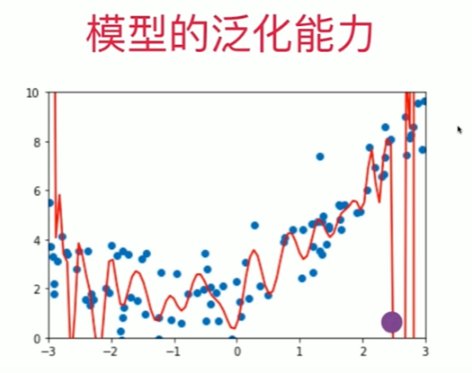
 1 [1]
 2 import numpy as np
 3 import matplotlib.pyplot as plt
 4 [2]
 5 x = np.random.uniform(-3, 3, size=100)
 6 X = x.reshape(-1,1)
 7 y = 0.5 * x**2 + x + 2 + np.random.normal(0, 1, size=100)
 8 [3]
 9 plt.scatter(X, y)
10 <matplotlib.collections.PathCollection at 0x2a05e646850>
11
12 [4]
13 from sklearn.linear_model import LinearRegression
14
15 lin_reg = LinearRegression()
16 lin_reg.fit(X,y)
17 lin_reg.score(X,y)
18 0.40801505133573723
19 [5]
20 y_predict = lin_reg.predict(X)
21 plt.scatter(X, y)
22 plt.plot(x, y_predict, color='r')
23 [<matplotlib.lines.Line2D at 0x2a061057bb0>]
24
25 [6]
26 from sklearn.metrics import mean_squared_error
27
28 y_predict = lin_reg.predict(X)
29 mean_squared_error(y,y_predict)
30 2.9187245186308566
31 使用多项式回归
32 [7]
33 from sklearn.pipeline import Pipeline
34 from sklearn.preprocessing import PolynomialFeatures
35 from sklearn.preprocessing import StandardScaler
36
37 def PolynomialRegression(degree):
38     return Pipeline([
39     ("poly",PolynomialFeatures(degree=degree)),#!!!!!!!!!
40     ("std_scaler",StandardScaler()),
41     ("lin_reg",LinearRegression())
42 ])
43 [8]
44 poly2_reg = PolynomialRegression(degree=2)
45 poly2_reg.fit(X,y)
46 Pipeline(steps=[('poly', PolynomialFeatures()),
47                 ('std_scaler', StandardScaler()),
48                 ('lin_reg', LinearRegression())])
49 [9]
50 y2_predict = poly2_reg.predict(X)
51 mean_squared_error(y,y2_predict)
52 0.8399501409780341
53 [10]
54 plt.scatter(X, y)
55 plt.plot(np.sort(x), y2_predict[np.argsort(x)], color='r')
56 [<matplotlib.lines.Line2D at 0x2a0610f9130>]
57
58 [11]
59 poly10_reg = PolynomialRegression(degree=10)
60 poly10_reg.fit(X,y)
61
62 y10_predict = poly10_reg.predict(X)
63 mean_squared_error(y,y10_predict)
64 0.7755990046397335
65 [12]
66 plt.scatter(X, y)
67 plt.plot(np.sort(x), y10_predict[np.argsort(x)], color='r')
68 [<matplotlib.lines.Line2D at 0x2a061166040>]
69
70 [13]
71 poly100_reg = PolynomialRegression(degree=100)
72 poly100_reg.fit(X,y)
73
74 y100_predict = poly100_reg.predict(X)
75 mean_squared_error(y,y100_predict)
76 0.46706858760890346
77 [14]
78 plt.scatter(X, y)
79 plt.plot(np.sort(x), y100_predict[np.argsort(x)], color='r')
80 [<matplotlib.lines.Line2D at 0x2a0611bde50>]
81
82 [15]
83 X_plot = np.linspace(-3, 3, 100).reshape(100,1)
84 y_plot = poly100_reg.predict(X_plot)
85
86 plt.scatter(x,y)
87 plt.plot(X_plot[:,0],y_plot,color='r')
88 [<matplotlib.lines.Line2D at 0x2a06122bfa0>]
89
90 [16]
91 X_plot = np.linspace(-3, 3, 100).reshape(100,1)
92 y_plot = poly100_reg.predict(X_plot)
93 plt.axis([-3, 3, -1,10])
94 plt.scatter(x,y)
95 plt.plot(X_plot[:,0],y_plot,color='r')
96 [<matplotlib.lines.Line2D at 0x2a06129fa00>]
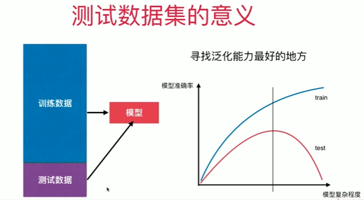
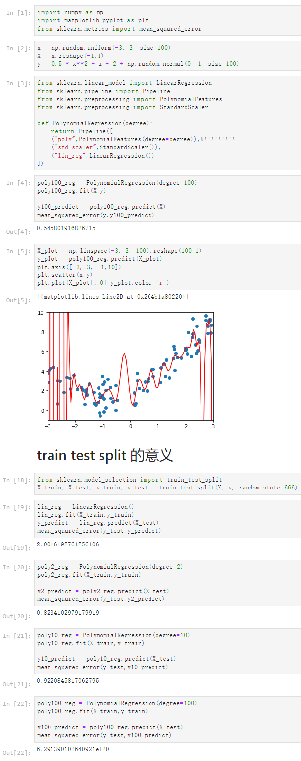
8-4 为什么要训练数据集与测试数据集

Notbook 示例
Notbook 源码
 1 [1]
 2 import numpy as np
 3 import matplotlib.pyplot as plt
 4 from sklearn.metrics import mean_squared_error
 5 [2]
 6 x = np.random.uniform(-3, 3, size=100)
 7 X = x.reshape(-1,1)
 8 y = 0.5 * x**2 + x + 2 + np.random.normal(0, 1, size=100)
 9 [3]
10 from sklearn.linear_model import LinearRegression
11 from sklearn.pipeline import Pipeline
12 from sklearn.preprocessing import PolynomialFeatures
13 from sklearn.preprocessing import StandardScaler
14
15 def PolynomialRegression(degree):
16     return Pipeline([
17     ("poly",PolynomialFeatures(degree=degree)),#!!!!!!!!!
18     ("std_scaler",StandardScaler()),
19     ("lin_reg",LinearRegression())
20 ])
21 [4]
22 poly100_reg = PolynomialRegression(degree=100)
23 poly100_reg.fit(X,y)
24
25 y100_predict = poly100_reg.predict(X)
26 mean_squared_error(y,y100_predict)
27 0.545801916826715
28 [5]
29 X_plot = np.linspace(-3, 3, 100).reshape(100,1)
30 y_plot = poly100_reg.predict(X_plot)
31 plt.axis([-3, 3, -1,10])
32 plt.scatter(x,y)
33 plt.plot(X_plot[:,0],y_plot,color='r')
34 [<matplotlib.lines.Line2D at 0x264b1a80220>]
35
36 train test split 的意义
37 [18]
38 from sklearn.model_selection import train_test_split
39 X_train, X_test, y_train, y_test = train_test_split(X, y, random_state=666)
40 [19]
41 lin_reg = LinearRegression()
42 lin_reg.fit(X_train,y_train)
43 y_predict = lin_reg.predict(X_test)
44 mean_squared_error(y_test,y_predict)
45 2.0016192761256106
46 [20]
47 poly2_reg = PolynomialRegression(degree=2)
48 poly2_reg.fit(X_train,y_train)
49
50 y2_predict = poly2_reg.predict(X_test)
51 mean_squared_error(y_test,y2_predict)
52 0.8234102979179919
53 [21]
54 poly10_reg = PolynomialRegression(degree=10)
55 poly10_reg.fit(X_train,y_train)
56
57 y10_predict = poly10_reg.predict(X_test)
58 mean_squared_error(y_test,y10_predict)
59 0.9220845817062795
60 [22]
61 poly100_reg = PolynomialRegression(degree=100)
62 poly100_reg.fit(X_train,y_train)
63
64 y100_predict = poly100_reg.predict(X_test)
65 mean_squared_error(y_test,y100_predict)
66 6.291390102640921e+20
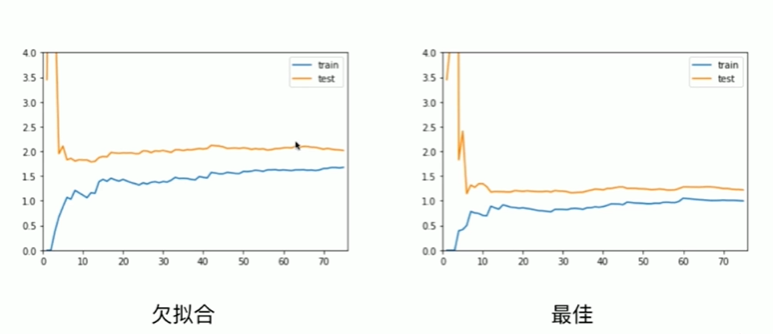
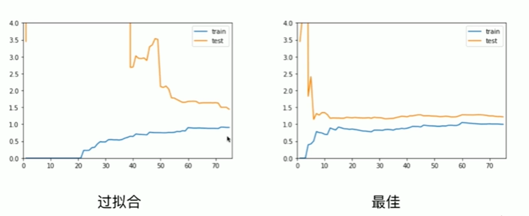
8-5 学习曲线

Notbook 示例
Notbook 源码
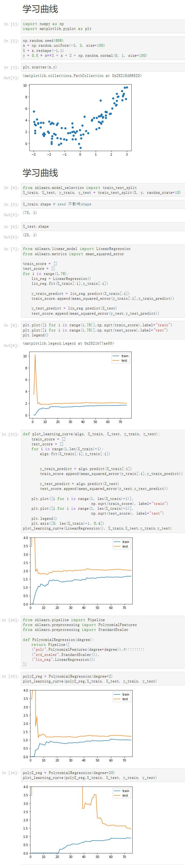
 1 学习曲线
 2 [1]
 3 import numpy as np
 4 import matplotlib.pyplot as plt
 5 [2]
 6 np.random.seed(666)
 7 x = np.random.uniform(-3, 3, size=100)
 8 X = x.reshape(-1,1)
 9 y = 0.5 * x**2 + x + 2 + np.random.normal(0, 1, size=100)
10 [3]
11 plt.scatter(x,y)
12 <matplotlib.collections.PathCollection at 0x28218d66820>
13
14 学习曲线
15 [4]
16 from sklearn.model_selection import train_test_split
17 X_train, X_test, y_train, y_test = train_test_split(X, y, random_state=10)
18 [5]
19 X_train.shape # seed 不影响shape
20 (75, 1)
21 [6]
22 X_test.shape
23 (25, 1)
24 [7]
25 from sklearn.linear_model import LinearRegression
26 from sklearn.metrics import mean_squared_error
27
28 train_score = []
29 test_score = []
30 for i in range(1,76):
31     lin_reg = LinearRegression()
32     lin_reg.fit(X_train[:i],y_train[:i])
33
34     y_train_predict = lin_reg.predict(X_train[:i])
35     train_score.append(mean_squared_error(y_train[:i],y_train_predict))
36
37     y_test_predict = lin_reg.predict(X_test)
38     test_score.append(mean_squared_error(y_test,y_test_predict))
39 [8]
40 plt.plot([i for i in range(1,76)],np.sqrt(train_score),label="train")
41 plt.plot([i for i in range(1,76)],np.sqrt(test_score),label="test")
42 plt.legend()
43 <matplotlib.legend.Legend at 0x2821b77ae50>
44
45 [13]
46 def plot_learning_curve(algo, X_train, X_test, y_train, y_test):
47     train_score = []
48     test_score = []
49     for i in range(1,len(X_train)+1):
50         algo.fit(X_train[:i],y_train[:i])
51
52
53         y_train_predict = algo.predict(X_train[:i])
54         train_score.append(mean_squared_error(y_train[:i],y_train_predict))
55
56         y_test_predict = algo.predict(X_test)
57         test_score.append(mean_squared_error(y_test,y_test_predict))
58
59     plt.plot([i for i in range(1, len(X_train)+1)],
60                                 np.sqrt(train_score), label="train")
61     plt.plot([i for i in range(1, len(X_train)+1)],
62                                 np.sqrt(test_score), label="test")
63     plt.legend()
64     plt.axis([0, len(X_train)+1, 0,4])
65 plot_learning_curve(LinearRegression(), X_train,X_test,y_train,y_test)
66
67 [14]
68 from sklearn.pipeline import Pipeline
69 from sklearn.preprocessing import PolynomialFeatures
70 from sklearn.preprocessing import StandardScaler
71
72 def PolynomialRegression(degree):
73     return Pipeline([
74     ("poly",PolynomialFeatures(degree=degree)),#!!!!!!!!!
75     ("std_scaler",StandardScaler()),
76     ("lin_reg",LinearRegression())
77 ])
78 [15]
79 poly2_reg = PolynomialRegression(degree=2)
80 plot_learning_curve(poly2_reg,X_train, X_test, y_train, y_test)
81
82 [16]
83 poly2_reg = PolynomialRegression(degree=20)
84 plot_learning_curve(poly2_reg,X_train, X_test, y_train, y_test)


 浙公网安备 33010602011771号