第6章梯度下降法

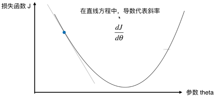
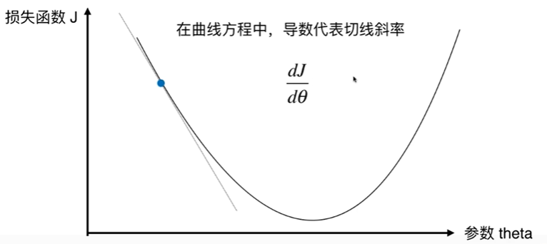
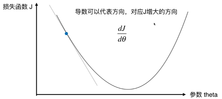
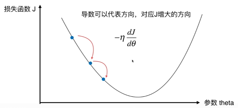
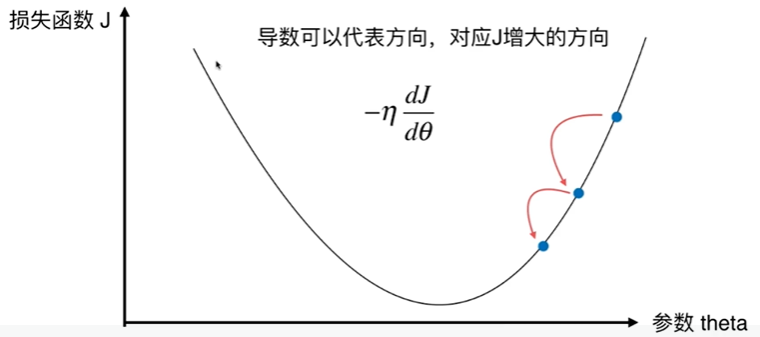
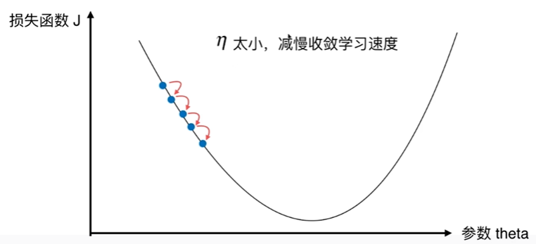
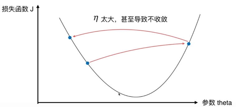
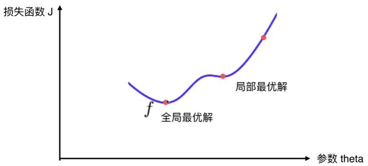
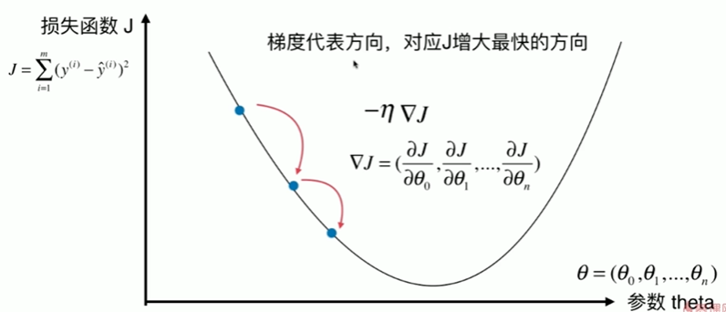
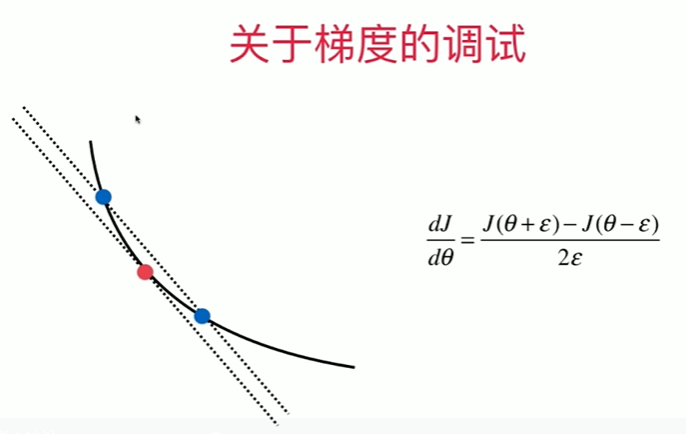
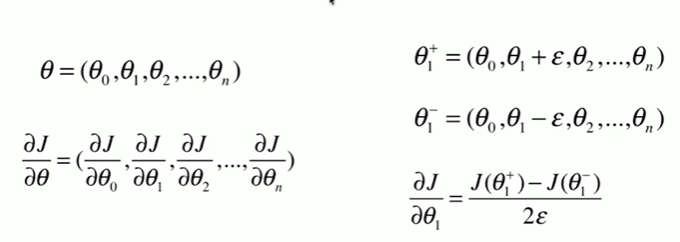
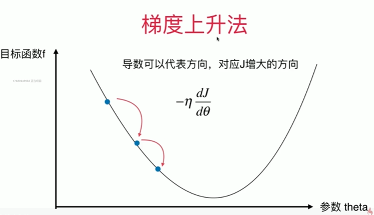
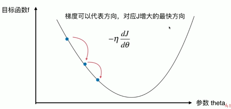
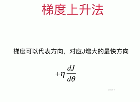
6-1 什么是梯度下降法

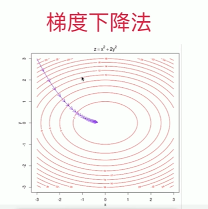
6-2 模拟实现梯度下降法

Notbook 示例

Notbook 源码

  1 [1]
  2 import numpy as np
  3 import matplotlib.pyplot as plt
  4 [2]
  5 plot_x = np.linspace(-1,6,141)
  6 plot_x
  7 array([-1.  , -0.95, -0.9 , -0.85, -0.8 , -0.75, -0.7 , -0.65, -0.6 ,
  8        -0.55, -0.5 , -0.45, -0.4 , -0.35, -0.3 , -0.25, -0.2 , -0.15,
  9        -0.1 , -0.05,  0.  ,  0.05,  0.1 ,  0.15,  0.2 ,  0.25,  0.3 ,
 10         0.35,  0.4 ,  0.45,  0.5 ,  0.55,  0.6 ,  0.65,  0.7 ,  0.75,
 11         0.8 ,  0.85,  0.9 ,  0.95,  1.  ,  1.05,  1.1 ,  1.15,  1.2 ,
 12         1.25,  1.3 ,  1.35,  1.4 ,  1.45,  1.5 ,  1.55,  1.6 ,  1.65,
 13         1.7 ,  1.75,  1.8 ,  1.85,  1.9 ,  1.95,  2.  ,  2.05,  2.1 ,
 14         2.15,  2.2 ,  2.25,  2.3 ,  2.35,  2.4 ,  2.45,  2.5 ,  2.55,
 15         2.6 ,  2.65,  2.7 ,  2.75,  2.8 ,  2.85,  2.9 ,  2.95,  3.  ,
 16         3.05,  3.1 ,  3.15,  3.2 ,  3.25,  3.3 ,  3.35,  3.4 ,  3.45,
 17         3.5 ,  3.55,  3.6 ,  3.65,  3.7 ,  3.75,  3.8 ,  3.85,  3.9 ,
 18         3.95,  4.  ,  4.05,  4.1 ,  4.15,  4.2 ,  4.25,  4.3 ,  4.35,
 19         4.4 ,  4.45,  4.5 ,  4.55,  4.6 ,  4.65,  4.7 ,  4.75,  4.8 ,
 20         4.85,  4.9 ,  4.95,  5.  ,  5.05,  5.1 ,  5.15,  5.2 ,  5.25,
 21         5.3 ,  5.35,  5.4 ,  5.45,  5.5 ,  5.55,  5.6 ,  5.65,  5.7 ,
 22         5.75,  5.8 ,  5.85,  5.9 ,  5.95,  6.  ])
 23 [3]
 24 plot_y = (plot_x - 2.5) ** 2 - 1
 25 [4]
 26 plt.plot(plot_x,plot_y)
 27 [<matplotlib.lines.Line2D at 0x1f6ec44cc70>]
 28 
 29 [5]
 30 def dJ(theta):
 31     return 2 * (theta - 2.5)
 32 [6]
 33 def J(theta):
 34     return (theta - 2.5) ** 2 - 1
 35 [7]
 36 eta = 0.1
 37 epsilon = 1e-8
 38 
 39 theta = 0.0
 40 while True:
 41     gradient = dJ(theta)
 42     last_theta = theta
 43     theta = theta - eta * gradient
 44     
 45     if(abs(dJ(theta)-dJ(last_theta)) < epsilon ):
 46         break
 47         
 48 print(theta)
 49 print(J(theta))
 50 2.4999999819074863
 51 -0.9999999999999997
 52 
 53 [8]
 54 theta = 0.0
 55 theta_history = [theta]
 56 while True:
 57     gradient = dJ(theta)
 58     last_theta = theta
 59     theta = theta - eta * gradient
 60     theta_history.append(theta)
 61     
 62     if(abs(dJ(theta)-dJ(last_theta)) < epsilon ):
 63         break
 64         
 65 plt.plot(plot_x,J(plot_x))
 66 plt.plot(np.array(theta_history),J(np.array(theta_history)),color = 'r',marker = '+')
 67 [<matplotlib.lines.Line2D at 0x1f6ec55d280>]
 68 
 69 [9]
 70 theta
 71 2.4999999819074863
 72 [10]
 73 len(theta_history) # 非46
 74 85
 75 [11]
 76 def gradient_descent(initial_theta, eta, epsilon = 1e-8):
 77     theta = initial_theta
 78     theta_history.append(initial_theta)
 79     
 80     while True:
 81         gradient = dJ(theta)
 82         last_theta = theta
 83         theta = theta - eta * gradient
 84         theta_history.append(theta)
 85     
 86         if(abs(dJ(theta)-dJ(last_theta)) < epsilon ):
 87             break
 88         
 89 def plot_theta_history():
 90     plt.plot(plot_x,J(plot_x))
 91     plt.plot(np.array(theta_history),J(np.array(theta_history)),color = 'r',marker = '+')
 92 [12]
 93 eta = 0.01
 94 theta_history = [] # theta_history[] = [] 错误
 95 gradient_descent(0.0,eta)
 96 plot_theta_history()
 97 
 98 [13]
 99 len(theta_history) # 非424
100 800
101 [14]
102 eta = 0.001
103 theta_history = [] 
104 gradient_descent(0.0,eta)
105 plot_theta_history()
106 
107 [15]
108 theta
109 2.4999999819074863
110 [16]
111 len(theta_history) # 3682
112 6903
113 [17]
114 eta = 0.8
115 theta_history = [] 
116 gradient_descent(0.0,eta)
117 plot_theta_history()
118 
119 [18]
120 len(theta_history)
121 43
122 [19]
123 theta
124 2.4999999819074863
125 eta = 1.1 theta_history = [] gradient_descent(0.0,eta) plot_theta_history()
126 
127 [20]
128 def J(theta):
129     try:
130         return (theta - 2.5) ** 2 - 1
131     except:
132         return float('inf')
133 [21]
134 def gradient_descent(initial_theta, eta,n_iters = 1e3, epsilon = 1e-8):
135     theta = initial_theta
136     theta_history.append(initial_theta)
137     i_iters = 0
138     
139     while i_iters < n_iters:
140         gradient = dJ(theta)
141         last_theta = theta
142         theta = theta - eta * gradient
143         theta_history.append(theta)
144     
145         if(abs(dJ(theta)-dJ(last_theta)) < epsilon ):
146             break
147         i_iters +=1
148         
149 def plot_theta_history():
150     plt.plot(plot_x,J(plot_x))
151     plt.plot(np.array(theta_history),J(np.array(theta_history)),color = 'r',marker = '+')
152 [22]
153 eta = 1.1 
154 theta_history = []
155 gradient_descent(0.0,eta) 
156 plot_theta_history()
157 
158 [23]
159 theta
160 2.4999999819074863
161 [24]
162 len(theta_history)
163 1001
164 [25]
165 dJ(theta_history[-1])
166 -7.58955044586262e+79
167 [26]
168 theta_history[-1]
169 -3.79477522293131e+79
170 [27]
171 np.argsort(theta)
172 array([0], dtype=int64)
173 [28]
174 eta = 1.1 
175 theta_history = []
176 gradient_descent(0.0,eta,n_iters=10) 
177 plot_theta_history()
178 
179 [29]
180 theta
181 2.4999999819074863

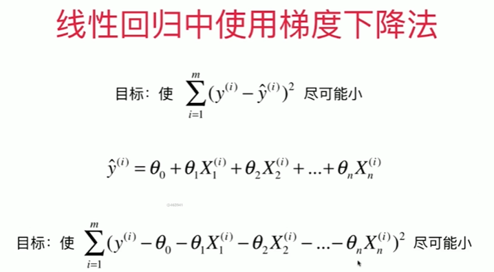
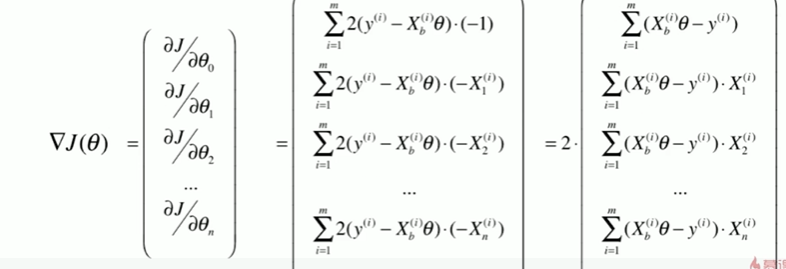
6-3 线性回归中的梯度下降法

6-4 实现线性回归中的梯度下降法

Notbook 示例

Notbook 源码

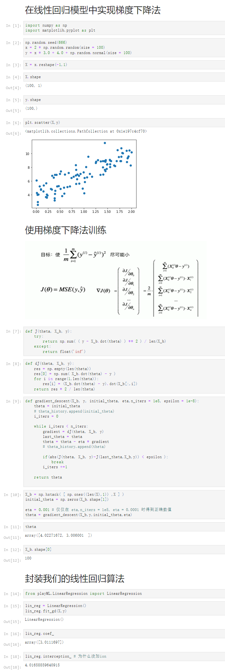
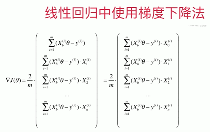
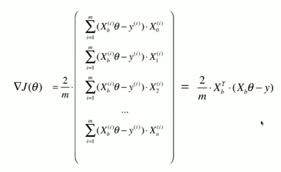
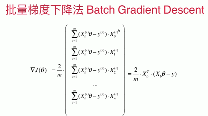
 1 在线性回归模型中实现梯度下降法
 2 [1]
 3 import numpy as np
 4 import matplotlib.pyplot as plt
 5 [2]
 6 np.random.seed(666)
 7 x = 2 * np.random.random(size = 100)
 8 y = x * 3.0 + 4.0 + np.random.normal(size = 100)
 9 [3]
10 X = x.reshape(-1,1)
11 [4]
12 X.shape
13 (100, 1)
14 [5]
15 y.shape
16 (100,)
17 [6]
18 plt.scatter(X,y)
19 <matplotlib.collections.PathCollection at 0x1e197c4cf70>
20 
21 使用梯度下降法训练
22 %E6%A2%AF%E5%BA%A6%E4%B8%8B%E9%99%8D.png
23 
24 [7]
25 def J(theta, X_b, y):
26     try:
27         return np.sum( ( y - X_b.dot(theta) ) ** 2 ) / len(X_b)
28     except:
29         return float('inf')
30 [8]
31 def dJ(theta, X_b, y):
32     res = np.empty(len(theta))
33     res[0] = np.sum( X_b.dot(theta) - y )
34     for i in range(1,len(theta)):
35         res[i] = (X_b.dot(theta) - y).dot(X_b[:,i])
36     return res * 2 / len(theta)
37 [9]
38 def gradient_descent(X_b, y, initial_theta, eta,n_iters = 1e5, epsilon = 1e-8):
39     theta = initial_theta
40     # theta_history.append(initial_theta)
41     i_iters = 0
42     
43     while i_iters < n_iters:
44         gradient = dJ(theta, X_b, y)
45         last_theta = theta
46         theta = theta - eta * gradient
47         # theta_history.append(theta)
48     
49         if(abs(J(theta, X_b, y)-J(last_theta,X_b,y)) < epsilon ):
50             break
51         i_iters +=1
52         
53     return theta
54         
55 [10]
56 X_b = np.hstack( [ np.ones((len(X),1)) ,X ] )
57 initial_theta = np.zeros(X_b.shape[1])
58 
59 eta = 0.001 # 仅仅在 eta,n_iters = 1e5, eta = 0.0001 时得到正确数值
60 theta = gradient_descent(X_b,y,initial_theta,eta)
61 [11]
62 theta
63 array([4.02271672, 3.006001  ])
64 [12]
65 X_b.shape[0]
66 100
67 封装我们的线性回归算法
68 [14]
69 from playML.LinearRegression import LinearRegression
70 [15]
71 lin_reg = LinearRegression()
72 lin_reg.fit_gd(X,y)
73 LinearRegression()
74 [16]
75 lin_reg.coef_
76 array([3.0111697])
77 [18]
78 lin_reg.interception_ # 为什么没加ion
79 4.01658859640915

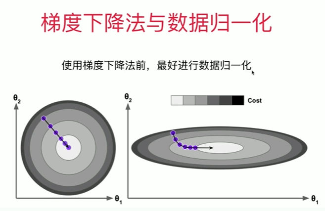
6-5 梯度下降的向量化和数据标准化

Notbook 示例

Notbook 源码

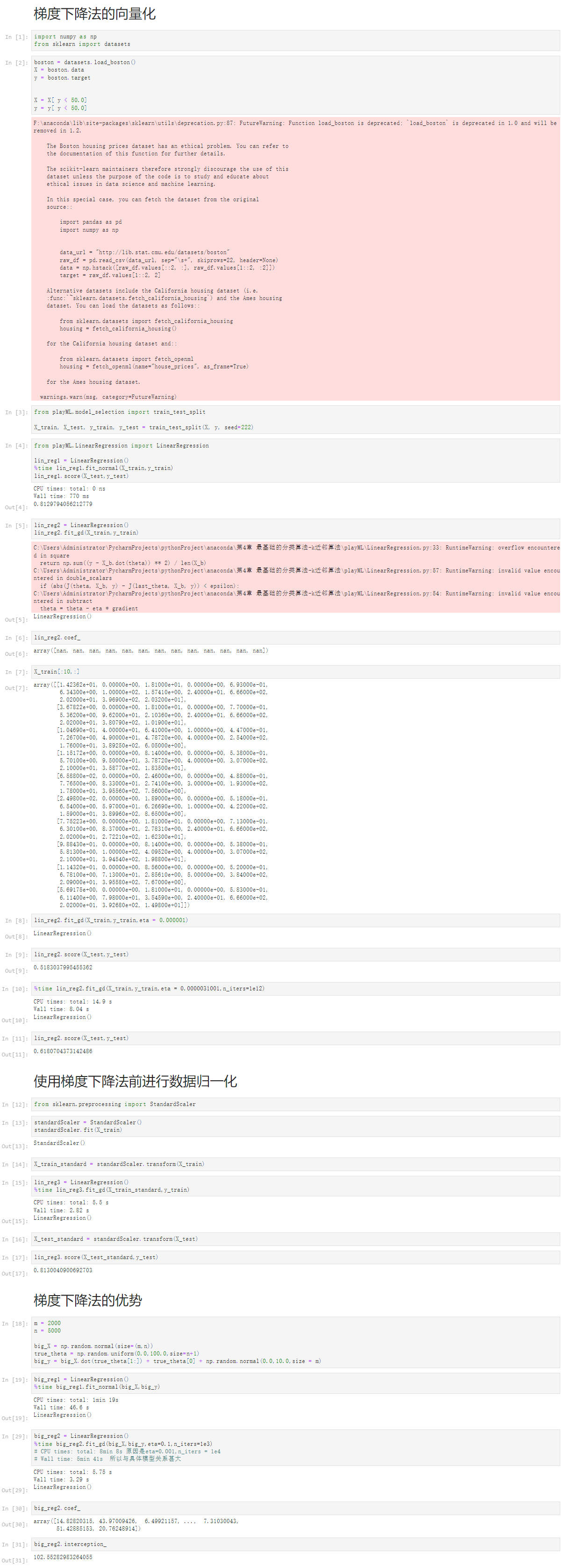
  1 梯度下降法的向量化
  2 [1]
  3 import numpy as np
  4 from sklearn import datasets
  5 [2]
  6 boston = datasets.load_boston()
  7 X = boston.data
  8 y = boston.target
  9 
 10 
 11 X = X[ y < 50.0]
 12 y = y[ y < 50.0]
 13 F:\anaconda\lib\site-packages\sklearn\utils\deprecation.py:87: FutureWarning: Function load_boston is deprecated; `load_boston` is deprecated in 1.0 and will be removed in 1.2.
 14 
 15     The Boston housing prices dataset has an ethical problem. You can refer to
 16     the documentation of this function for further details.
 17 
 18     The scikit-learn maintainers therefore strongly discourage the use of this
 19     dataset unless the purpose of the code is to study and educate about
 20     ethical issues in data science and machine learning.
 21 
 22     In this special case, you can fetch the dataset from the original
 23     source::
 24 
 25         import pandas as pd
 26         import numpy as np
 27 
 28 
 29         data_url = "http://lib.stat.cmu.edu/datasets/boston"
 30         raw_df = pd.read_csv(data_url, sep="\s+", skiprows=22, header=None)
 31         data = np.hstack([raw_df.values[::2, :], raw_df.values[1::2, :2]])
 32         target = raw_df.values[1::2, 2]
 33 
 34     Alternative datasets include the California housing dataset (i.e.
 35     :func:`~sklearn.datasets.fetch_california_housing`) and the Ames housing
 36     dataset. You can load the datasets as follows::
 37 
 38         from sklearn.datasets import fetch_california_housing
 39         housing = fetch_california_housing()
 40 
 41     for the California housing dataset and::
 42 
 43         from sklearn.datasets import fetch_openml
 44         housing = fetch_openml(name="house_prices", as_frame=True)
 45 
 46     for the Ames housing dataset.
 47     
 48   warnings.warn(msg, category=FutureWarning)
 49 
 50 [3]
 51 from playML.model_selection import train_test_split
 52 
 53 X_train, X_test, y_train, y_test = train_test_split(X, y, seed=222)
 54 [4]
 55 from playML.LinearRegression import LinearRegression
 56 
 57 lin_reg1 = LinearRegression()
 58 %time lin_reg1.fit_normal(X_train,y_train)
 59 lin_reg1.score(X_test,y_test)
 60 CPU times: total: 0 ns
 61 Wall time: 770 ms
 62 
 63 0.8129794056212779
 64 [5]
 65 lin_reg2 = LinearRegression()
 66 lin_reg2.fit_gd(X_train,y_train)
 67 C:\Users\Administrator\PycharmProjects\pythonProject\anaconda\第4章 最基础的分类算法-k近邻算法\playML\LinearRegression.py:33: RuntimeWarning: overflow encountered in square
 68   return np.sum((y - X_b.dot(theta)) ** 2) / len(X_b)
 69 C:\Users\Administrator\PycharmProjects\pythonProject\anaconda\第4章 最基础的分类算法-k近邻算法\playML\LinearRegression.py:57: RuntimeWarning: invalid value encountered in double_scalars
 70   if (abs(J(theta, X_b, y) - J(last_theta, X_b, y)) < epsilon):
 71 C:\Users\Administrator\PycharmProjects\pythonProject\anaconda\第4章 最基础的分类算法-k近邻算法\playML\LinearRegression.py:54: RuntimeWarning: invalid value encountered in subtract
 72   theta = theta - eta * gradient
 73 
 74 LinearRegression()
 75 [6]
 76 lin_reg2.coef_
 77 array([nan, nan, nan, nan, nan, nan, nan, nan, nan, nan, nan, nan, nan])
 78 [7]
 79 X_train[:10,:]
 80 array([[1.42362e+01, 0.00000e+00, 1.81000e+01, 0.00000e+00, 6.93000e-01,
 81         6.34300e+00, 1.00000e+02, 1.57410e+00, 2.40000e+01, 6.66000e+02,
 82         2.02000e+01, 3.96900e+02, 2.03200e+01],
 83        [3.67822e+00, 0.00000e+00, 1.81000e+01, 0.00000e+00, 7.70000e-01,
 84         5.36200e+00, 9.62000e+01, 2.10360e+00, 2.40000e+01, 6.66000e+02,
 85         2.02000e+01, 3.80790e+02, 1.01900e+01],
 86        [1.04690e-01, 4.00000e+01, 6.41000e+00, 1.00000e+00, 4.47000e-01,
 87         7.26700e+00, 4.90000e+01, 4.78720e+00, 4.00000e+00, 2.54000e+02,
 88         1.76000e+01, 3.89250e+02, 6.05000e+00],
 89        [1.15172e+00, 0.00000e+00, 8.14000e+00, 0.00000e+00, 5.38000e-01,
 90         5.70100e+00, 9.50000e+01, 3.78720e+00, 4.00000e+00, 3.07000e+02,
 91         2.10000e+01, 3.58770e+02, 1.83500e+01],
 92        [6.58800e-02, 0.00000e+00, 2.46000e+00, 0.00000e+00, 4.88000e-01,
 93         7.76500e+00, 8.33000e+01, 2.74100e+00, 3.00000e+00, 1.93000e+02,
 94         1.78000e+01, 3.95560e+02, 7.56000e+00],
 95        [2.49800e-02, 0.00000e+00, 1.89000e+00, 0.00000e+00, 5.18000e-01,
 96         6.54000e+00, 5.97000e+01, 6.26690e+00, 1.00000e+00, 4.22000e+02,
 97         1.59000e+01, 3.89960e+02, 8.65000e+00],
 98        [7.75223e+00, 0.00000e+00, 1.81000e+01, 0.00000e+00, 7.13000e-01,
 99         6.30100e+00, 8.37000e+01, 2.78310e+00, 2.40000e+01, 6.66000e+02,
100         2.02000e+01, 2.72210e+02, 1.62300e+01],
101        [9.88430e-01, 0.00000e+00, 8.14000e+00, 0.00000e+00, 5.38000e-01,
102         5.81300e+00, 1.00000e+02, 4.09520e+00, 4.00000e+00, 3.07000e+02,
103         2.10000e+01, 3.94540e+02, 1.98800e+01],
104        [1.14320e-01, 0.00000e+00, 8.56000e+00, 0.00000e+00, 5.20000e-01,
105         6.78100e+00, 7.13000e+01, 2.85610e+00, 5.00000e+00, 3.84000e+02,
106         2.09000e+01, 3.95580e+02, 7.67000e+00],
107        [5.69175e+00, 0.00000e+00, 1.81000e+01, 0.00000e+00, 5.83000e-01,
108         6.11400e+00, 7.98000e+01, 3.54590e+00, 2.40000e+01, 6.66000e+02,
109         2.02000e+01, 3.92680e+02, 1.49800e+01]])
110 [8]
111 lin_reg2.fit_gd(X_train,y_train,eta = 0.000001)
112 LinearRegression()
113 [9]
114 lin_reg2.score(X_test,y_test)
115 0.5183037995455362
116 [10]
117 %time lin_reg2.fit_gd(X_train,y_train,eta = 0.0000031001,n_iters=1e12)
118 CPU times: total: 14.9 s
119 Wall time: 8.04 s
120 
121 LinearRegression()
122 [11]
123 lin_reg2.score(X_test,y_test)
124 0.6180704373142486
125 使用梯度下降法前进行数据归一化
126 [12]
127 from sklearn.preprocessing import StandardScaler
128 [13]
129 standardScaler = StandardScaler()
130 standardScaler.fit(X_train)
131 StandardScaler()
132 [14]
133 X_train_standard = standardScaler.transform(X_train)
134 [15]
135 lin_reg3 = LinearRegression()
136 %time lin_reg3.fit_gd(X_train_standard,y_train)
137 CPU times: total: 5.5 s
138 Wall time: 2.82 s
139 
140 LinearRegression()
141 [16]
142 X_test_standard = standardScaler.transform(X_test)
143 [17]
144 lin_reg3.score(X_test_standard,y_test)
145 0.8130040900692703
146 梯度下降法的优势
147 [18]
148 m = 2000
149 n = 5000
150 
151 big_X = np.random.normal(size=(m,n))
152 true_theta = np.random.uniform(0.0,100.0,size=n+1)
153 big_y = big_X.dot(true_theta[1:]) + true_theta[0] + np.random.normal(0.0,10.0,size = m)
154 [19]
155 big_reg1 = LinearRegression()
156 %time big_reg1.fit_normal(big_X,big_y)
157 CPU times: total: 1min 19s
158 Wall time: 46.6 s
159 
160 LinearRegression()
161 [29]
162 big_reg2 = LinearRegression()
163 %time big_reg2.fit_gd(big_X,big_y,eta=0.1,n_iters=1e3)
164 # CPU times: total: 8min 8s 原因是eta=0.001,n_iters = 1e4
165 # Wall time: 5min 41s  所以与具体模型关系甚大
166 CPU times: total: 5.75 s
167 Wall time: 3.29 s
168 
169 LinearRegression()
170 [30]
171 big_reg2.coef_
172 array([14.82820315, 43.97009426,  6.49921157, ...,  7.31030043,
173        51.42885153, 20.76248914])
174 [31]
175 big_reg2.interception_
176 102.55282983264055

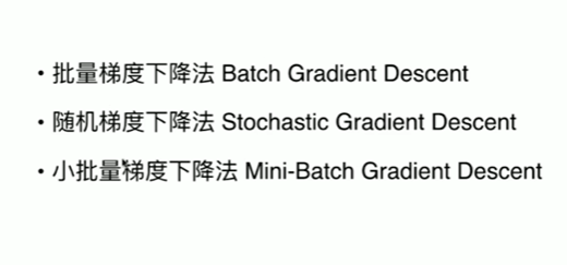
6-6 随机梯度下降法

Notbook 示例

Notbook 源码

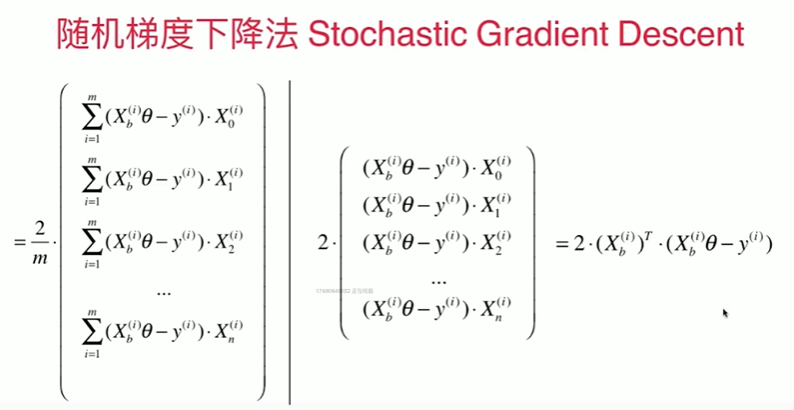
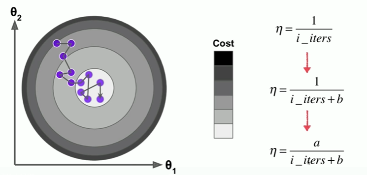
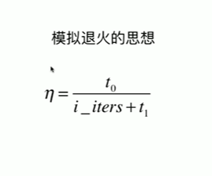
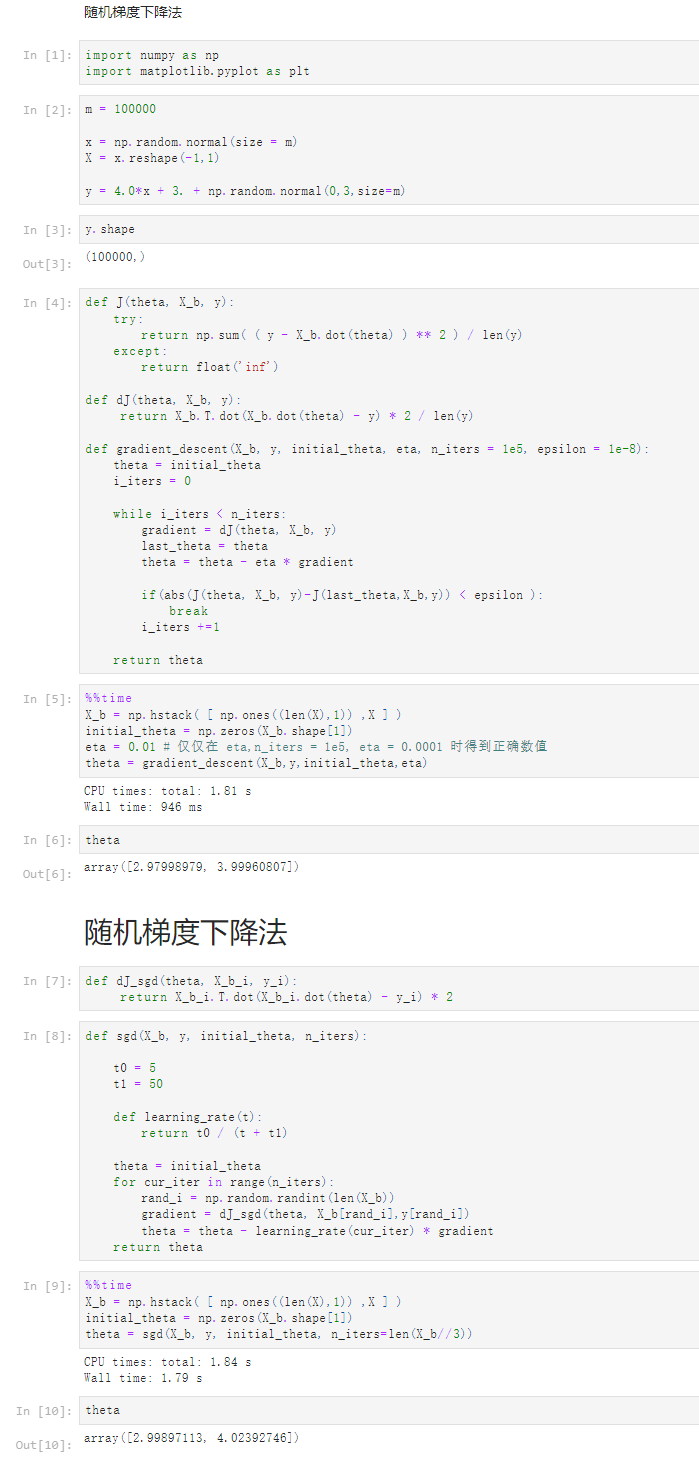
 1 随机梯度下降法
 2 
 3 [1]
 4 import numpy as np
 5 import matplotlib.pyplot as plt
 6 [2]
 7 m = 100000
 8 
 9 x = np.random.normal(size = m)
10 X = x.reshape(-1,1)
11 
12 y = 4.0*x + 3. + np.random.normal(0,3,size=m)
13 [3]
14 y.shape
15 (100000,)
16 [4]
17 def J(theta, X_b, y):
18     try:
19         return np.sum( ( y - X_b.dot(theta) ) ** 2 ) / len(y)
20     except:
21         return float('inf')
22     
23 def dJ(theta, X_b, y):
24      return X_b.T.dot(X_b.dot(theta) - y) * 2 / len(y)
25     
26 def gradient_descent(X_b, y, initial_theta, eta, n_iters = 1e5, epsilon = 1e-8):
27     theta = initial_theta
28     i_iters = 0
29     
30     while i_iters < n_iters:
31         gradient = dJ(theta, X_b, y)
32         last_theta = theta
33         theta = theta - eta * gradient
34         
35         if(abs(J(theta, X_b, y)-J(last_theta,X_b,y)) < epsilon ):
36             break
37         i_iters +=1
38         
39     return theta
40 [5]
41 %%time
42 X_b = np.hstack( [ np.ones((len(X),1)) ,X ] )
43 initial_theta = np.zeros(X_b.shape[1])
44 eta = 0.01 # 仅仅在 eta,n_iters = 1e5, eta = 0.0001 时得到正确数值
45 theta = gradient_descent(X_b,y,initial_theta,eta)
46 CPU times: total: 1.81 s
47 Wall time: 946 ms
48 
49 [6]
50 theta
51 array([2.97998979, 3.99960807])
52 随机梯度下降法
53 [7]
54 def dJ_sgd(theta, X_b_i, y_i):
55      return X_b_i.T.dot(X_b_i.dot(theta) - y_i) * 2
56 [8]
57 def sgd(X_b, y, initial_theta, n_iters):
58     
59     t0 = 5
60     t1 = 50
61     
62     def learning_rate(t):
63         return t0 / (t + t1)
64     
65     theta = initial_theta
66     for cur_iter in range(n_iters):
67         rand_i = np.random.randint(len(X_b))
68         gradient = dJ_sgd(theta, X_b[rand_i],y[rand_i])
69         theta = theta - learning_rate(cur_iter) * gradient
70     return theta
71 [9]
72 %%time
73 X_b = np.hstack( [ np.ones((len(X),1)) ,X ] )
74 initial_theta = np.zeros(X_b.shape[1])
75 theta = sgd(X_b, y, initial_theta, n_iters=len(X_b//3))
76 CPU times: total: 1.84 s
77 Wall time: 1.79 s
78 
79 [10]
80 theta
81 array([2.99897113, 4.02392746])

6-7 scikit-learn中的随机梯度下降法

Notbook 示例

Notbook 源码

  1 使用我们自己的SGD
  2 [1]
  3 import numpy as np 
  4 import matplotlib.pyplot as plt
  5 [2]
  6 m = 100000
  7 
  8 x = np.random.normal(size = m)
  9 X = x.reshape(-1,1)
 10 
 11 y = 4.0*x + 3. + np.random.normal(0,3,size=m)
 12 [3]
 13 from playML.LinearRegression import LinearRegression
 14 
 15 lin_reg = LinearRegression()
 16 lin_reg.fit_sgd(X, y, n_iters=2)
 17 LinearRegression()
 18 [4]
 19 lin_reg._theta
 20 array([3.01202028, 3.97799884])
 21 [5]
 22 lin_reg.coef_
 23 array([3.97799884])
 24 [6]
 25 lin_reg.interception_
 26 3.012020275313304
 27 真实使用我们自己的SGD
 28 [7]
 29 from sklearn import datasets
 30 
 31 boston = datasets.load_boston()
 32 X = boston.data
 33 y = boston.target
 34 
 35 
 36 X = X[ y < 50.0]
 37 y = y[ y < 50.0]
 38 F:\anaconda\lib\site-packages\sklearn\utils\deprecation.py:87: FutureWarning: Function load_boston is deprecated; `load_boston` is deprecated in 1.0 and will be removed in 1.2.
 39 
 40     The Boston housing prices dataset has an ethical problem. You can refer to
 41     the documentation of this function for further details.
 42 
 43     The scikit-learn maintainers therefore strongly discourage the use of this
 44     dataset unless the purpose of the code is to study and educate about
 45     ethical issues in data science and machine learning.
 46 
 47     In this special case, you can fetch the dataset from the original
 48     source::
 49 
 50         import pandas as pd
 51         import numpy as np
 52 
 53 
 54         data_url = "http://lib.stat.cmu.edu/datasets/boston"
 55         raw_df = pd.read_csv(data_url, sep="\s+", skiprows=22, header=None)
 56         data = np.hstack([raw_df.values[::2, :], raw_df.values[1::2, :2]])
 57         target = raw_df.values[1::2, 2]
 58 
 59     Alternative datasets include the California housing dataset (i.e.
 60     :func:`~sklearn.datasets.fetch_california_housing`) and the Ames housing
 61     dataset. You can load the datasets as follows::
 62 
 63         from sklearn.datasets import fetch_california_housing
 64         housing = fetch_california_housing()
 65 
 66     for the California housing dataset and::
 67 
 68         from sklearn.datasets import fetch_openml
 69         housing = fetch_openml(name="house_prices", as_frame=True)
 70 
 71     for the Ames housing dataset.
 72     
 73   warnings.warn(msg, category=FutureWarning)
 74 
 75 [8]
 76 from playML.model_selection import train_test_split
 77 
 78 X_train, X_test, y_train, y_test = train_test_split(X, y, seed=666) # 666 效果比 222 好很多
 79 [9]
 80 from sklearn.preprocessing import StandardScaler
 81 
 82 standardScaler = StandardScaler()
 83 standardScaler.fit(X_train)
 84 X_train_standard = standardScaler.transform(X_train)
 85 X_test_standard = standardScaler.transform(X_test)
 86 [10]
 87 from playML.LinearRegression import LinearRegression
 88 
 89 lin_reg2 = LinearRegression()
 90 %time lin_reg2.fit_sgd(X_train_standard, y_train, n_iters=2)
 91 lin_reg2.score(X_test_standard,y_test)
 92 CPU times: total: 15.6 ms
 93 Wall time: 8.98 ms
 94 
 95 0.7911189802097699
 96 [11]
 97 %time lin_reg2.fit_sgd(X_train_standard, y_train, n_iters=50)
 98 lin_reg2.score(X_test_standard,y_test)
 99 CPU times: total: 219 ms
100 Wall time: 226 ms
101 
102 0.8132588958621522
103 [13]
104 %time lin_reg2.fit_sgd(X_train_standard, y_train, n_iters=500)
105 lin_reg2.score(X_test_standard,y_test)
106 CPU times: total: 2.09 s
107 Wall time: 2.93 s
108 
109 0.8129564757875579
110 scikit-learn 中的SGD
111 [14]
112 from sklearn.linear_model import SGDRegressor
113 [15]
114 sgd_reg = SGDRegressor()
115 %time sgd_reg.fit(X_train_standard,y_train)
116 sgd_reg.score(X_test_standard,y_test)
117 CPU times: total: 0 ns
118 Wall time: 116 ms
119 
120 0.8129895569490898
121 [18]
122 sgd_reg = SGDRegressor(n_iter_no_change=100)# n_iter 报错 
123 %time sgd_reg.fit(X_train_standard,y_train)
124 sgd_reg.score(X_test_standard,y_test)
125 CPU times: total: 15.6 ms
126 Wall time: 22.9 ms
127 
128 0.8131520202077357

6-8 如何确定梯度计算的准确性调试梯度下降法

Notbook 示例

Notbook 源码

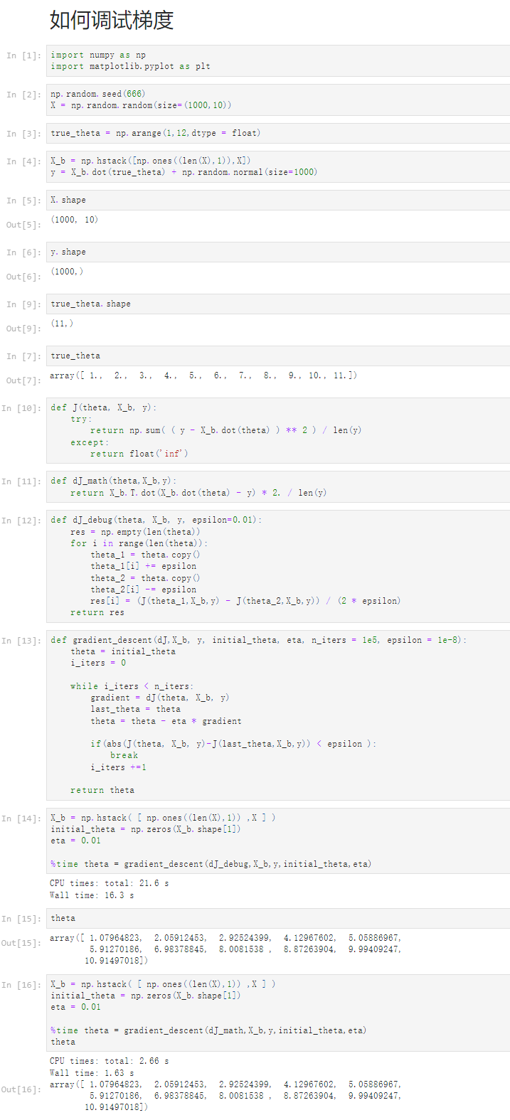
 1 如何调试梯度
 2 [1]
 3 import numpy as np
 4 import matplotlib.pyplot as plt
 5 [2]
 6 np.random.seed(666)
 7 X = np.random.random(size=(1000,10))
 8 [3]
 9 true_theta = np.arange(1,12,dtype = float)
10 [4]
11 X_b = np.hstack([np.ones((len(X),1)),X])
12 y = X_b.dot(true_theta) + np.random.normal(size=1000)
13 [5]
14 X.shape
15 (1000, 10)
16 [6]
17 y.shape
18 (1000,)
19 [9]
20 true_theta.shape
21 (11,)
22 [7]
23 true_theta
24 array([ 1.,  2.,  3.,  4.,  5.,  6.,  7.,  8.,  9., 10., 11.])
25 [10]
26 def J(theta, X_b, y):
27     try:
28         return np.sum( ( y - X_b.dot(theta) ) ** 2 ) / len(y)
29     except:
30         return float('inf')
31 [11]
32 def dJ_math(theta,X_b,y):
33     return X_b.T.dot(X_b.dot(theta) - y) * 2. / len(y)
34 [12]
35 def dJ_debug(theta, X_b, y, epsilon=0.01):
36     res = np.empty(len(theta))
37     for i in range(len(theta)):
38         theta_1 = theta.copy()
39         theta_1[i] += epsilon
40         theta_2 = theta.copy()
41         theta_2[i] -= epsilon
42         res[i] = (J(theta_1,X_b,y) - J(theta_2,X_b,y)) / (2 * epsilon)
43     return res
44 [13]
45 def gradient_descent(dJ,X_b, y, initial_theta, eta, n_iters = 1e5, epsilon = 1e-8):
46     theta = initial_theta
47     i_iters = 0
48     
49     while i_iters < n_iters:
50         gradient = dJ(theta, X_b, y)
51         last_theta = theta
52         theta = theta - eta * gradient
53         
54         if(abs(J(theta, X_b, y)-J(last_theta,X_b,y)) < epsilon ):
55             break
56         i_iters +=1
57         
58     return theta
59 [14]
60 X_b = np.hstack( [ np.ones((len(X),1)) ,X ] )
61 initial_theta = np.zeros(X_b.shape[1])
62 eta = 0.01 
63 
64 %time theta = gradient_descent(dJ_debug,X_b,y,initial_theta,eta)
65 CPU times: total: 21.6 s
66 Wall time: 16.3 s
67 
68 [15]
69 theta
70 array([ 1.07964823,  2.05912453,  2.92524399,  4.12967602,  5.05886967,
71         5.91270186,  6.98378845,  8.0081538 ,  8.87263904,  9.99409247,
72        10.91497018])
73 [16]
74 X_b = np.hstack( [ np.ones((len(X),1)) ,X ] )
75 initial_theta = np.zeros(X_b.shape[1])
76 eta = 0.01 
77 
78 %time theta = gradient_descent(dJ_math,X_b,y,initial_theta,eta)
79 theta
80 CPU times: total: 2.66 s
81 Wall time: 1.63 s
82 
83 array([ 1.07964823,  2.05912453,  2.92524399,  4.12967602,  5.05886967,
84         5.91270186,  6.98378845,  8.0081538 ,  8.87263904,  9.99409247,
85        10.91497018])