Algorithm: Polynomial Multiplication -- Fast Fourier Transform / Number-Theoretic Transform (English version)
Intro:
This blog will start with plain multiplication, go through Divide-and-conquer multiplication, and reach FFT and NTT.
The aim is to enable the reader (and myself) to fully understand the idea.
Template question entrance: Luogu P3803 【模板】多项式乘法(FFT)
Plain multiplication
Assumption: Two polynomials are \(A(x)=\sum_{i=0}^{n}a_ix^i,B(x)=\sum_{i=0}^{m}b_ix^i\)
Prerequisite knowledge:
Knowledge of junior high school mathematics
The simplest method is to multiply term by term and then combine like terms, written as the formula:
If \(C(x)=A(x)B(x)\), then \(C(x)=\sum_{i=0}^{n+m}c_ix^i\), where \(c_i=\sum_{j=0}^ia_jb_{i-j}\).
So a plain multiplication is generated, see the code (\(b\) array omitted with some useless techniques).
//This program is written by Brian Peng.
#pragma GCC optimize("Ofast","inline","no-stack-protector")
#include<bits/stdc++.h>
using namespace std;
#define Rd(a) (a=read())
#define Gc(a) (a=getchar())
#define Pc(a) putchar(a)
int read(){
	register int x;register char c(getchar());register bool k;
	while(!isdigit(c)&&c^'-')if(Gc(c)==EOF)exit(0);
	if(c^'-')k=1,x=c&15;else k=x=0;
	while(isdigit(Gc(c)))x=(x<<1)+(x<<3)+(c&15);
	return k?x:-x;
}
void wr(register int a){
	if(a<0)Pc('-'),a=-a;
	if(a<=9)Pc(a|'0');
	else wr(a/10),Pc((a%10)|'0');
}
signed const INF(0x3f3f3f3f),NINF(0xc3c3c3c3);
long long const LINF(0x3f3f3f3f3f3f3f3fLL),LNINF(0xc3c3c3c3c3c3c3c3LL);
#define Ps Pc(' ')
#define Pe Pc('\n')
#define Frn0(i,a,b) for(register int i(a);i<(b);++i)
#define Frn1(i,a,b) for(register int i(a);i<=(b);++i)
#define Frn_(i,a,b) for(register int i(a);i>=(b);--i)
#define Mst(a,b) memset(a,b,sizeof(a))
#define File(a) freopen(a".in","r",stdin),freopen(a".out","w",stdout)
#define N (2000010)
int n,m,a[N],b,c[N];
signed main(){
	Rd(n),Rd(m);
	Frn1(i,0,n)Rd(a[i]);
	Frn1(i,0,m){Rd(b);Frn1(j,0,n)c[i+j]+=b*a[j];}
	Frn1(i,0,n+m)wr(c[i]),Ps;
	exit(0);
}
Time complexity: \(O(nm)\) (If\(m=O(n)\), then \(O(n^2)\))
Memory complexity: \(O(n)\)
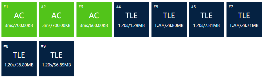
Results:

Expected, so we need to optimize it.
Divide-and-conquer multiplication (Fake)
P.s This part describes the Divide-and-conquer method of FFT, which is still different from the exact FFT, so you can skip it if you have already mastered the Divide-and-conquer idea.
Let \(n\) be the smallest positive integer power of \(2\) that is strictly greater than both the degrees of \(A(x),B(x)\), and we write \(A(x)=\sum_{i=0}^{n-1}a_ix^i,B(x)=\sum_{i=0}^{n-1}b_ix^i\), where the unexisted coefficients are made \(0\).
Prerequisite knowledge:
The idea of Divide-and-conquer
Now consider how to optimize multiplication.
Try to separate two polynomials according to the parity of the index of \(x\):
\(A(x)=A^{[0]}(x^2)+xA^{[1]}(x^2),B(x)=B^{[0]}(x^2)+xB^{[1]}(x^2)\),
where \(A^{[0]}(x)=\sum_{i=0}^{n/2-1}a_{2i}x^i,A^{[1]}(x)=\sum_{i=0}^{n/2-1}a_{2i+1}x^i\), and \(B^{[0]}(x)\) and \(B^{[1]}(x)\) are similar.
Therefore, the two polynomials are split into four polynomials, each with degree \(<n/2\).
We let \(A=A(x),A^{[0]}=A^{[0]}(x^2),A^{[1]}=A^{[1]}(x^2)\), and similar for \(B\) and others,
then \(AB=(A^{[0]}+xA^{[1]})(B^{[0]}+xB^{[1]})=A^{[0]}B^{[0]}+x(A^{[1]}B^{[0]}+A^{[0]}B^{[1]})+x^2A^{[1]}B^{[1]}\).
A Divide-and-conquer algorithm can be found here: split two polynomials in half, then recursively do \(4\) polynomial multiplications, and finally combine them together (polynomial addition is \(O(n)\) anyway)
P.s As \(A^{[0]}=A^{[0]}(x^2)\) and \(A^{[1]}=A^{[1]}(x^2)\), the combination process is alternating. Here is the code. (In the code, the \(n\) above is replaced by the variable s, and vector is used to save memory)
//This program is written by Brian Peng.
#pragma GCC optimize("Ofast","inline","no-stack-protector")
#include<bits/stdc++.h>
using namespace std;
#define Rd(a) (a=read())
#define Gc(a) (a=getchar())
#define Pc(a) putchar(a)
int read(){
	register int x;register char c(getchar());register bool k;
	while(!isdigit(c)&&c^'-')if(Gc(c)==EOF)exit(0);
	if(c^'-')k=1,x=c&15;else k=x=0;
	while(isdigit(Gc(c)))x=(x<<1)+(x<<3)+(c&15);
	return k?x:-x;
}
void wr(register int a){
	if(a<0)Pc('-'),a=-a;
	if(a<=9)Pc(a|'0');
	else wr(a/10),Pc((a%10)|'0');
}
signed const INF(0x3f3f3f3f),NINF(0xc3c3c3c3);
long long const LINF(0x3f3f3f3f3f3f3f3fLL),LNINF(0xc3c3c3c3c3c3c3c3LL);
#define Ps Pc(' ')
#define Pe Pc('\n')
#define Frn0(i,a,b) for(register int i(a);i<(b);++i)
#define Frn1(i,a,b) for(register int i(a);i<=(b);++i)
#define Frn_(i,a,b) for(register int i(a);i>=(b);--i)
#define Mst(a,b) memset(a,b,sizeof(a))
#define File(a) freopen(a".in","r",stdin),freopen(a".out","w",stdout)
typedef vector<int> Vct;
int n,m,s;
Vct a,b,c;
void add(Vct&a,Vct&b,Vct&c){Frn0(i,0,c.size())c[i]=a[i]+b[i];}
void mlt(Vct&a,Vct&b,Vct&c,int n);
signed main(){
	Rd(n),Rd(m),a.resize(s=1<<int(log2(max(n,m))+1)),b.resize(s),c.resize(s<<1);
	Frn1(i,0,n)Rd(a[i]);
	Frn1(i,0,m)Rd(b[i]);
	mlt(a,b,c,s);
	Frn1(i,0,n+m)wr(c[i]),Ps;
	exit(0);
}
void mlt(Vct&a,Vct&b,Vct&c,int n){
	int n2(n>>1);
	Vct a0(n2),a1(n2),b0(n2),b1(n2),ab0(n),ab1(n),abm(n);
	if(n==1){c[0]=a[0]*b[0];return;}
	Frn0(i,0,n2)a0[i]=a[i<<1],a1[i]=a[i<<1|1],b0[i]=b[i<<1],b1[i]=b[i<<1|1];
	mlt(a0,b0,ab0,n2),mlt(a1,b1,ab1,n2);
	Frn0(i,0,n)c[i<<1]=ab0[i]+(i?ab1[i-1]:0);
	mlt(a0,b1,ab0,n2),mlt(a1,b0,ab1,n2),add(ab0,ab1,abm);
	Frn0(i,0,n-1)c[i<<1|1]=abm[i];
}
Results:
even worse
Why's that? Because the Time complexity is still \(O(n^2)\).
\(\textit{Proof. } T(n)=4T(n/2)+f(n)\), in which \(f(n)=O(n)\) the time complexity of polynomial addition.
Using the Master Theorem with \(a=4,b=2,\log_ba=\log_2 4=2>1\), we have \(T(n)=O(n^{\log_ba})=O(n^2)\).
So, let's continue optimizing
Divide-and-conquer multiplication (Real)
Let's consider how to optimize the "fake" one.
An intro question: Try to find an algorithm to multiply linear expressions \(ax+b\) and \(cx+d\) with only \(3\) multiplication steps.
Let's expand the multiplication: \((ax+b)(cx+d)=acx^2+(ad+bc)x+bd\), there seems to be \(4\) multiplication steps used.
Hence, if we can only use \(3\) multiplication steps, then \(ad+bc\) should cost only one.
Let's add all coefficients together: \(ac+ad+bc+bd=(a+b)(c+d)\),
and here is the answer! Use \(3\) multiplication steps to calculate \(ac,bd,(a+b)(c+d)\) respectively, and the \(x\) coefficient is just \(ad+bc=(a+b)(c+d)-ac-bd\)
Let's go back to the original question
As \(AB=(A^{[0]}+xA^{[1]})(B^{[0]}+xB^{[1]})=A^{[0]}B^{[0]}+x(A^{[1]}B^{[0]}+A^{[0]}B^{[1]})+x^2A^{[1]}B^{[1]}\),
we can use the similar method to reduce one multiplication step: \(A^{[1]}B^{[0]}+A^{[0]}B^{[1]}=(A^{[0]}+A^{[1]})(B^{[0]}+B^{[1]})-A^{[0]}B^{[0]}-A^{[1]}B^{[1]}\)
Here is the code:
//This program is written by Brian Peng.
#pragma GCC optimize("Ofast","inline","no-stack-protector")
#include<bits/stdc++.h>
using namespace std;
#define Rd(a) (a=read())
#define Gc(a) (a=getchar())
#define Pc(a) putchar(a)
int read(){
	register int x;register char c(getchar());register bool k;
	while(!isdigit(c)&&c^'-')if(Gc(c)==EOF)exit(0);
	if(c^'-')k=1,x=c&15;else k=x=0;
	while(isdigit(Gc(c)))x=(x<<1)+(x<<3)+(c&15);
	return k?x:-x;
}
void wr(register int a){
	if(a<0)Pc('-'),a=-a;
	if(a<=9)Pc(a|'0');
	else wr(a/10),Pc((a%10)|'0');
}
signed const INF(0x3f3f3f3f),NINF(0xc3c3c3c3);
long long const LINF(0x3f3f3f3f3f3f3f3fLL),LNINF(0xc3c3c3c3c3c3c3c3LL);
#define Ps Pc(' ')
#define Pe Pc('\n')
#define Frn0(i,a,b) for(register int i(a);i<(b);++i)
#define Frn1(i,a,b) for(register int i(a);i<=(b);++i)
#define Frn_(i,a,b) for(register int i(a);i>=(b);--i)
#define Mst(a,b) memset(a,b,sizeof(a))
#define File(a) freopen(a".in","r",stdin),freopen(a".out","w",stdout)
typedef vector<int> Vct;
int n,m,s;
Vct a,b,c;
void add(Vct&a,Vct&b,Vct&c){Frn0(i,0,c.size())c[i]=a[i]+b[i];}
void mns(Vct&a,Vct&b,Vct&c){Frn0(i,0,c.size())c[i]=a[i]-b[i];}
void mlt(Vct&a,Vct&b,Vct&c);
signed main(){
	Rd(n),Rd(m),a.resize(s=1<<int(log2(max(n,m))+1)),b.resize(s),c.resize(s<<1);
	Frn1(i,0,n)Rd(a[i]);
	Frn1(i,0,m)Rd(b[i]);
	mlt(a,b,c);
	Frn1(i,0,n+m)wr(c[i]),Ps;
	exit(0);
}
void mlt(Vct&a,Vct&b,Vct&c){
	int n(a.size()),n2(a.size()>>1);
	Vct a0(n2),a1(n2),b0(n2),b1(n2),ab0(n),ab1(n),abm(n);
	if(n==1){c[0]=a[0]*b[0];return;}
	Frn0(i,0,n2)a0[i]=a[i<<1],a1[i]=a[i<<1|1],b0[i]=b[i<<1],b1[i]=b[i<<1|1];
	mlt(a0,b0,ab0),mlt(a1,b1,ab1);
	Frn0(i,0,n)c[i<<1]=ab0[i]+(i?ab1[i-1]:0);
	add(a0,a1,a0),add(b0,b1,b0),mlt(a0,b0,abm),mns(abm,ab0,abm),mns(abm,ab1,abm);
	Frn0(i,0,n-1)c[i<<1|1]=abm[i];
}
Results

Better than fake DC multiplication, but even worse than plain multiplication...
Let's calculate the time complexity of this algorithm:
\(T(n)=3T(n/2)+f(n)\), in which \(f(n)=O(n)\).
Using Master Theorem with \(a=3,b=2,\log_ba=\log_2 3\approx1.58>1\), so \(T(n)=O(n^{\log_ba})=O(n^{\log_2 3})\).
Hmm...so why is it even worse than plain multiplication?
Reason 1. The constant factor of DC multiplication is too high.
Reason 2. In \(\#5\) test case, we have \(n=1,m=3\cdot 10^6\), then \(O(n^{\log_2 3})\) is really worse than \(O(nm)\)...
So, our FFT is eventually coming!
Fast Fourier Transform
Fairly Frightening Transform
Let \(n\) be the smallest positive integer power of \(2\) greater than \(\deg A(x)+\deg B(x)\) and we write \(A(x)=\sum_{i=0}^{n-1}a_ix^i,B(x)=\sum_{i=0}^{n-1}b_ix^i\).
Prerequisite knowledge:
The idea of Divide-and-conquer
Complex number basics
Linear algebra basics (not strictly required)
Part 1: To representations of the polynomial
1. Coefficient expressions
For a polynomial \(A(x)=\sum_{i=0}^{n-1}a_ix^i\), its coefficient expression is a vector \(\pmb{a}=\left[\begin{matrix}a_0\\a_1\\\vdots\\a_{n-1}\end{matrix} \right]\)
In coefficient expressions, the time complexities of the following methods are:
-
Evaluation at a point: \(O(n)\)
-
Addition: \(O(n)\)
-
Multiplication: plain \(O(n^2)\), DC \((n^{\log_2 3})\)
P.s When calculating polynomial multiplication \(C(x)=A(x)B(x)\), the corresponding coefficient expression \(\pmb{c}\) is defined as the convolution of \(\pmb{a}\) and \(\pmb{b}\), written as \(\pmb{c}=\pmb{a}\bigotimes\pmb{b}\).
2. Point-valued expressions
The point-valued expression of a polynomial \(A(x)\) with \(\deg A<n\) is a set of \(n\) points: \(\{(x_0,y_0),(x_1,y_1),\cdots,(x_{n-1},y_{n-1})\}\)
We can use \(n\) evaluations to convert a coefficient expression to a point-valued expression with a list of \((x_0,x_1,\cdots,x_{n-1})\) in time complexity of \(O(n^2)\) as shown:
\(\left[\begin{matrix}1&x_0&x_0^2&\cdots&x_0^{n-1}\\1&x_1&x_1^2&\cdots&x_1^{n-1}\\\vdots&\vdots&\vdots&\ddots&\vdots\\1&x_{n-1}&x_{n-1}^2&\cdots&x_{n-1}^{n-1}\end{matrix} \right]\left[\begin{matrix}a_0\\a_1\\\vdots\\a_{n-1}\end{matrix} \right]=\left[\begin{matrix}y_0\\y_1\\\vdots\\y_{n-1}\end{matrix} \right]\)
The matrix is written as \(V(x_0,x_1,\cdots,x_{n-1})\), named Vandermonde matrix, so the formula is simplified to \(V(x_0,x_1,\cdots,x_{n-1})\pmb{a}=\pmb{y}\).
Using Lagrangian formulas, a point-valued expression can be converted back into a coefficient expression in \(O(n^2)\) time, a process called interpolation.
With two polynomials in point-valued expressions with the same list of \((x_0,\cdots,x_{n-1})\), the time complexity of following methods are:
-
Addition: \(O(n)\) (Adding the \(y_i\) value respectively)
-
Multiplication \(O(n)\) (similar)
This is one central idea of FFT powered polynomial multiplication: with carefully chosen \(x_i\) values, we can achieve evaluation in \(O(n\log n)\), multiplication in \(O(n)\), and finally interpolation in \(O(n\log n)\).
So what are those \(x_i\) values?
Part 2: Complex roots of unity
The \(n\)-th roots of unity are exactly \(n\) complex numbers \(\omega\) that satisfy \(\omega^n=1\), written as:
\(\omega_n^k=e^{2\pi ik/n}=\cos(2\pi k/n)+i\sin(2\pi k/n)\).
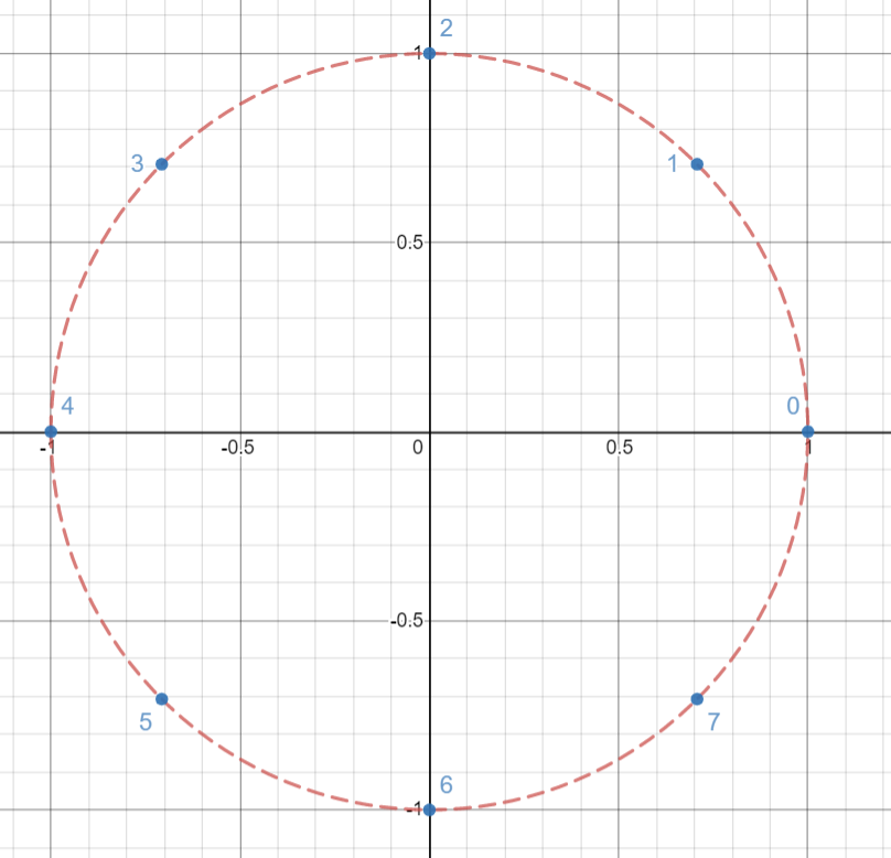
We can plot \(n\)-th roots of unity as \(n\) vertices of a regular \(n\)-gon inscribed in the unit circle on the complex plane. For example, the following graph shows the \(8\)-th roots of unity.
There is a pattern: \(\omega_n^j\omega_n^k=\omega_n^{j+k}=\omega_n^{(j+k)\mod n}\). Specifically, \(\omega_n^{-1}=\omega_n^{n-1}\).
Three other important lemmas.
\(\text{Lemma 1. }\) For all integers \(n\geqslant 0,k\geqslant 0,d>0\), we have \(\omega_{dn}^{dk}=\omega_n^k\).
\(\textit{Proof. }\omega_{dn}^{dk}=(e^{2\pi i/dn})^{dk}=(e^{2\pi i/n})^k=\omega_n^k.\square\)
\(\text{Lemma 2. }\) For all even number \(n\) and integer \(k\), we have \((\omega_n^k)^2=(\omega_n^{k+n/2})^2=\omega_{n/2}^k\).
\(\textit{Proof. }(\omega_n^k)^2=\omega_n^{2k},(\omega_n^{k+n/2})^2=\omega_n^{2k+n}=\omega_n^{2k}\). Lastly, \(\omega_n^{2k}=\omega_{n/2}^k\) by \(\text{Lemma 1}.\square\)
\(\text{Lemma 3. }\) For all integers \(n,k\geqslant 0\) such that \(n\nmid k\), we have \(\sum_{j=0}^{n-1}(\omega_n^k)^j=0\).
\(\textit{Proof. }\) When \(n\nmid k\), we have \(\omega_n^k\neq 1\), so \(\sum_{j=0}^{n-1}(\omega_n^k)^j=\frac{1-(\omega_n^k)^n}{1-\omega_n^k}=\frac{1-\omega_n^{nk}}{1-\omega_n^k}=\frac{1-1}{1-\omega_n^k}=0.\square\) (Question: why is \(n\nmid k\) necessary?)
The above properties of roots of unity are the essence of FFT optimization.
Part 3: Discrete Fourier Transform
Recall the definition of \(n\), which is a power of \(2\). DFT is just the evaluation of coefficient expressed \(A(x)\) on \(n\)-th roots of unity. We write the Vandermonde matrix as
\(V_n=V(\omega_n^0,\omega_n^1,\cdots,\omega_n^{n-1})=\left[\begin{matrix}1&1&1&1&\cdots&1\\1&\omega_n&\omega_n^2&\omega_n^3&\cdots&\omega_n^{n-1}\\1&\omega_n^2&\omega_n^4&\omega_n^6&\cdots&\omega_n^{2(n-1)}\\1&\omega_n^3&\omega_n^6&\omega_n^9&\cdots&\omega_n^{3(n-1)}\\\vdots&\vdots&\vdots&\vdots&\ddots&\vdots\\1&\omega_n^{n-1}&\omega_n^{2(n-1)}&\omega_n^{3(n-1)}&\cdots&\omega_n^{(n-1)(n-1)}\end{matrix} \right]\),
then the formula of DFT is \(\pmb{y}=\text{DFT}_n(\pmb a)\): \(V_n\pmb{a}=\pmb{y}\). Specifically, \(y_i=\sum_{j=0}^{n-1}[V_n]_{ij}a_j=\sum_{j=0}^{n-1}\omega_n^{ij}a_j\).
So, how can we achieve it in \(O(n\log n)\)?
Part 4: FFT
Like DC multiplication, we split the polynomial by parity: \(A(x)=A^{[0]}(x^2)+xA^{[1]}(x^2)\), where \(A^{[0]}(x)=\sum_{i=0}^{n/2-1}a_{2i}x^i,A^{[1]}(x)=\sum_{i=0}^{n/2-1}a_{2i+1}x^i\).
Then, our evaluation of \(A(x)\) on \(\omega_n^0,\omega_n^1,\cdots,\omega_n^{n-1}\) becomes
1. Divide-and-conquer: evaluating \(A^{[0]}(x)\) and \(A^{[1]}(x)\) on \((\omega_n^0)^2,(\omega_n^1)^2,\cdots,(\omega_n^{n-1})^2\).
By \(\text{Lemma 2}\), the list \((\omega_n^0)^2,(\omega_n^1)^2,\cdots,(\omega_n^{n-1})^2\) is exactly a repeated list of \(n/2\)-roots of unity (Why?)
So we can apply \(DFT_{n/2}(\pmb a^{[0]})=y^{[0]},DFT_{n/2}(\pmb a^{[1]})=\pmb y^{[1]}\). And the second step is
2. Combining the answers.
As \(\omega_n^{n/2}=e^{2\pi i (n/2)/n}=e^{\pi i}=-1\) (The beautiful Euler's formula!),
we have \(\omega_n^{k+n/2}=\omega_n^k\omega_n^{n/2}=-\omega_n^k\),
so \(y_i=y^{[0]}_i+\omega_n^i y^{[1]}_i,y_{i+n/2}=y^{[0]}_i-\omega_n^i y^{[1]}_i,\) for all \(i=0,1,\cdots,n/2-1\).
Specifically, when \(n=1\), \(\omega_1^0 a_0=a_0\) in the trivial case.
Let's calculate the time complexity
\(T(n)=2T(n/2)+f(n)\), in which \(f(n)=O(n)\) is the time used for combination.
Using Master Theorem with \(a=2,b=2,\log_ba=\log_2 2=1\), we have \(T(n)=O(n^{\log_ba}\log n)=O(n\log n)\). Whooo!
Part 5: Inverse DFT
Don't celebrate too soon, there is still interpolation. Awww
Since \(\pmb{y}=\text{DFT}_n(\pmb{a})=V_n\pmb{a}\), we have \(\pmb{a}=V_n^{-1}\pmb{y}\), written as \(\pmb{a}=\text{DFT}_n^{-1}(\pmb{y})\).
\(\text{Theorem. }\) For all \(i,j=0,1,\cdots,n-1\), we have \([V_n^{-1}]_{ij}=\omega_n^{-ij}/n\).
\(\textit{Proof. }\) We show that \(V_n^{-1}V_n=I_n\) the identity matrix:
\([V_n^{-1}V_n]_{ij}=\sum_{k=0}^{n-1}(\omega_n^{-ik}/n)\omega_n^{kj}=\frac{\sum_{k=0}^{n-1}\omega_n^{-ik}\omega_n^{kj}}{n}=\frac{\sum_{k=0}^{n-1}\omega_n^{(j-i)k}}{n}\)
If \(i=j\), then \(\frac{\sum_{k=0}^{n-1}\omega_n^0}{n}=n/n=1\). Otherwise, it is \(0/n=0\) by \(\text{Lemma 3}\). Therefore, \(I_n\) is formed. \(\square\)
Next, \(\pmb{a}=\text{DFT}_n^{-1}(\pmb{y})=V_n^{-1}\pmb{y}\), in which \(a_i=\sum_{j=0}^{n-1}[V_n^{-1}]_{ij}y_j=\sum_{j=0}^{n-1}(\omega_n^{-ij}/n)y_j=\frac{\sum_{j=0}^{n-1}\omega_n^{-ij}y_j}{n}\).
Let's compare: in DFT, \(y_i=\sum_{j=0}^{n-1}\omega_n^{ij}a_j\).
Therefore, we can convert DFT to IDFT by simply replacing \(\omega_n^k\) with \(\omega_n^{-k}\) and dividing the final answers by \(n\).
Part 6: Recursive Implementation
According to the previous text, we just need to modify the code of DC multiplication.
To save memory, we redistribute the coefficients of \(A^{[0]}\) to the left and \(A^{[1]}\) to the right.
In the code, o\(=\omega_n\), w\(=\omega_n^i\).
P.s Don't for get \(/n\) for IDFT. In the code, the +0.5 is used to improve accuracy for integer-coefficient FFT.
//This program is written by Brian Peng.
#pragma GCC optimize("Ofast","inline","no-stack-protector")
#include<bits/stdc++.h>
using namespace std;
#define Rd(a) (a=read())
#define Gc(a) (a=getchar())
#define Pc(a) putchar(a)
int read(){
	register int u;register char c(getchar());register bool k;
	while(!isdigit(c)&&c^'-')if(Gc(c)==EOF)exit(0);
	if(c^'-')k=1,u=c&15;else k=u=0;
	while(isdigit(Gc(c)))u=(u<<1)+(u<<3)+(c&15);
	return k?u:-u;
}
void wr(register int a){
	if(a<0)Pc('-'),a=-a;
	if(a<=9)Pc(a|'0');
	else wr(a/10),Pc((a%10)|'0');
}
signed const INF(0x3f3f3f3f),NINF(0xc3c3c3c3);
long long const LINF(0x3f3f3f3f3f3f3f3fLL),LNINF(0xc3c3c3c3c3c3c3c3LL);
#define Ps Pc(' ')
#define Pe Pc('\n')
#define Frn0(i,a,b) for(register int i(a);i<(b);++i)
#define Frn1(i,a,b) for(register int i(a);i<=(b);++i)
#define Frn_(i,a,b) for(register int i(a);i>=(b);--i)
#define Mst(a,b) memset(a,b,sizeof(a))
#define File(a) freopen(a".in","r",stdin),freopen(a".out","w",stdout)
double const Pi(acos(-1));
typedef complex<double> Cpx;
#define N (2100000)
Cpx o,w,a[N],b[N],tmp[N],x,y;
int n,m,s;
bool iv;
void fft(Cpx*a,int n);
signed main(){
	Rd(n),Rd(m),s=1<<int(log2(n+m)+1);
	Frn1(i,0,n)Rd(a[i]);
	Frn1(i,0,m)Rd(b[i]);
	fft(a,s),fft(b,s);
	Frn0(i,0,s)a[i]*=b[i];
	iv=1,fft(a,s);
	Frn1(i,0,n+m)wr(a[i].real()/s+0.5),Ps;
	exit(0);
}
void fft(Cpx*a,int n){
	if(n==1)return;
	int n2(n>>1);
	Frn0(i,0,n2)tmp[i]=a[i<<1],tmp[i+n2]=a[i<<1|1];
	copy(tmp,tmp+n,a),fft(a,n2),fft(a+n2,n2);
	o={cos(Pi/n2),(iv?-1:1)*sin(Pi/n2)},w=1;
	Frn0(i,0,n2)x=a[i],y=w*a[i+n2],a[i]=x+y,a[i+n2]=x-y,w*=o;
}
Time complexity: \(O(n\log n)\)
Memory complexity: \(O(n)\)
Results:
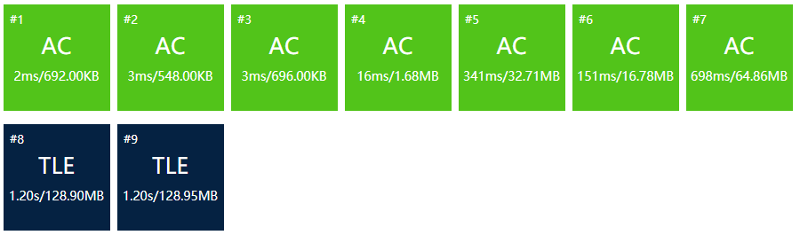
Not fully AC, as recursive implementation is not fast enough.
Part 6: Iterative Implementation
For \(n=\deg_A+1,m=\deg B+1\), let \(l=\lceil\log_2(n+m+1)\rceil\) and \(s=2^l\), then \(s\) is the "\(n\)" in previous parts.
Similarly, we redistribute the coefficients of \(A^{[0]}\) to the left and \(A^{[1]}\) to the right.
Observe the pattern of redistribution in each layer of recursion. Take \(s=8\) as an example:
0-> 0 1 2 3 4 5 6 7
1-> 0 2 4 6|1 3 5 7
2-> 0 4|2 6|1 5|3 7
end 0|4|2|6|1|5|3|7
Still confused? Write them in base-2:
0-> 000 001 010 011 100 101 110 111
1-> 000 010 100 110|001 011 101 111
2-> 000 100|010 110|001 101|011 111
end 000|100|010|110|001|101|011|111
The base-2 expressions are reversed in the last layer!
A hint of the proof: the redistribution is based on parity, which is equivalent to the last digit of base-2 expressions.
In the code, we use array \(r_{0..s-1}\) to store the reverse numbers.
Butterfly Operation
It is already written in the code of recursive implementation, but let's clarify that:
Still remember \(y_i=y^{[0]}_i+\omega_n^i y^{[1]}_i,y_{i+n/2}=y^{[0]}_i-\omega_n^i y^{[1]}_i,i=0,1,\cdots,n/2-1\)?
To save memory, we do not create the array \(\pmb y\), but the combination is done on the original location of the array \(\pmb a\).
After redistribution, we have \(a^{[0]}_i=a_i\) and \(a^{[1]}_i=a_{i+n/2}\).
Let \(x=a^{[0]}_i=a_i,y=\omega_n^i a^{[1]}_i=\omega_n^i a_{i+n/2}\),
then the result of DFT is simply \(a_i=x+y,a_{i+n/2}=x-y\)!
With Butterfly Operation, we just need to redistribute the coefficients according to \(r\), and then combine iteratively to implement FFT.
//This program is written by Brian Peng.
#pragma GCC optimize("Ofast","inline","no-stack-protector")
#include<bits/stdc++.h>
using namespace std;
#define Rd(a) (a=read())
#define Gc(a) (a=getchar())
#define Pc(a) putchar(a)
int read(){
	register int u;register char c(getchar());register bool k;
	while(!isdigit(c)&&c^'-')if(Gc(c)==EOF)exit(0);
	if(c^'-')k=1,u=c&15;else k=u=0;
	while(isdigit(Gc(c)))u=(u<<1)+(u<<3)+(c&15);
	return k?u:-u;
}
void wr(register int a){
	if(a<0)Pc('-'),a=-a;
	if(a<=9)Pc(a|'0');
	else wr(a/10),Pc((a%10)|'0');
}
signed const INF(0x3f3f3f3f),NINF(0xc3c3c3c3);
long long const LINF(0x3f3f3f3f3f3f3f3fLL),LNINF(0xc3c3c3c3c3c3c3c3LL);
#define Ps Pc(' ')
#define Pe Pc('\n')
#define Frn0(i,a,b) for(register int i(a);i<(b);++i)
#define Frn1(i,a,b) for(register int i(a);i<=(b);++i)
#define Frn_(i,a,b) for(register int i(a);i>=(b);--i)
#define Mst(a,b) memset(a,b,sizeof(a))
#define File(a) freopen(a".in","r",stdin),freopen(a".out","w",stdout)
double const Pi(acos(-1));
typedef complex<double> Cpx;
#define N (2100000)
Cpx a[N],b[N],o,w,x,y;
int n,m,l,s,r[N];
void fft(Cpx*a,bool iv);
signed main(){
	Rd(n),Rd(m),s=1<<(l=log2(n+m)+1);
	Frn1(i,0,n)Rd(a[i]);
	Frn1(i,0,m)Rd(b[i]);
	Frn0(i,0,s)r[i]=(r[i>>1]>>1)|((i&1)<<(l-1));
	fft(a,0),fft(b,0);
	Frn0(i,0,s)a[i]*=b[i];
	fft(a,1);
	Frn1(i,0,n+m)wr(a[i].real()+0.5),Ps;
	exit(0);
}
void fft(Cpx*a,bool iv){
	Frn0(i,0,s)if(i<r[i])swap(a[i],a[r[i]]);
	for(int i(2),i2(1);i<=s;i2=i,i<<=1){
		o={cos(Pi/i2),(iv?-1:1)*sin(Pi/i2)};
		for(int j(0);j<s;j+=i){
			w=1;
			Frn0(k,0,i2){
				x=a[j+k],y=w*a[j+k+i2];
				a[j+k]=x+y,a[j+k+i2]=x-y,w*=o;
			}
		}
	}
	if(iv)Frn0(i,0,s)a[i]/=s;
}
Time complexity: \(O(n\log n)\)
Memory complexity: \(O(n)\)
Results:
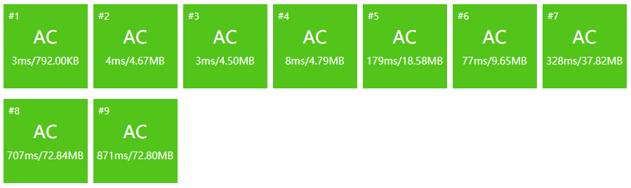
Celebrate
Extension: Number Theoretic Transform
Although FFT has excellent time complexity, inaccuracy will inevitably arise because of the use of complex numbers.
If the polynomial coefficients and results are non-negative integers in a certain range, NTT is a better choice on accuracy and speed.
Prerequisite knowledge:
FFT absolutely
Modular arithmetics basics
Primitive roots
Assume that the following calculations are in the context of \(\bmod P\), where \(P\) is a prime number.
For a positive integer \(g\), if the list of powers of \(g\) contains every positive integer \(<P\), then we call \(g\) a primitive root \(\bmod P\). (Digression: in Group Theory, the equivalence class of \(g\) in \(\Z_p\) is a generator of \(\Z_p^*\))
E.g For \(P=7\) and for all positive integers \(<P\), we calculate the possibilities of their powers.
1-> {1}
2-> {1,2,4}
3-> {1,2,3,4,5,6}
4-> {1,2,4}
5-> {1,2,3,4,5,6}
6-> {1,6}
Therefore, \(3,5\) are the primitive roots \(\bmod 7\).
In the code, we commonly use \(P=998244353,g=3\).
The special property of primitive root \(g\) is that its powers repeat with period \(P-1\).
E.g Let \(P=7,g=3\), then the powers of \(g\) (beginning with \(g^0\)) are:\(1,3,2,6,4,5,1,3,2,6,4,5,\cdots\).
This property is very similar to the roots of unity. If we take \(n=P-1\) and \(\omega_n=g\), then all three lemmas in the FFT part are satisfied.
However, to complete NTT, there is one last step.
The substitute for roots of unity
In FFT, we use \(n\)-th roots of unity, where \(n\) is a power of \(2\).
However, \(P-1\) is not necessarily \(n\). Hence, we cannot directly replace \(\omega_n\) with \(g\).
Now, as the powers of \(g\) have a period of \(P-1\),
if we take a factor \(k\) of \(P-1\), then the powers of \(g^k\) have a period of \(\frac{P-1}{k}\). (Why?)
This means that if we take \(k=\frac{P-1}{n}\), then the powers of \(g^k\) have a period of exactly \(n\).
But, how can we be sure that \(n\) is always a factor of \(P-1\)?
This is why we choose \(P=998244353\), as \(P-1=998244352=2^{23}\cdot 7\cdot 17\), with a high multiplicity of \(2\).
Therefore, \(g^{\frac{P-1}{n}}\) is just our substitute of \(\omega_n\).
In the code, we use \(g^{-1}=332748118\) and \(\cdot s^{-1}\) when doing IDFT. Make sure that you include \(\bmod P\) in every operation.
//This program is written by Brian Peng.
#pragma GCC optimize("Ofast","inline","no-stack-protector")
#include<bits/stdc++.h>
using namespace std;
#define int long long
#define Rd(a) (a=read())
#define Gc(a) (a=getchar())
#define Pc(a) putchar(a)
int read(){
	register int u;register char c(getchar());register bool k;
	while(!isdigit(c)&&c^'-')if(Gc(c)==EOF)exit(0);
	if(c^'-')k=1,u=c&15;else k=u=0;
	while(isdigit(Gc(c)))u=(u<<1)+(u<<3)+(c&15);
	return k?u:-u;
}
void wr(register int a){
	if(a<0)Pc('-'),a=-a;
	if(a<=9)Pc(a|'0');
	else wr(a/10),Pc((a%10)|'0');
}
signed const INF(0x3f3f3f3f),NINF(0xc3c3c3c3);
long long const LINF(0x3f3f3f3f3f3f3f3fLL),LNINF(0xc3c3c3c3c3c3c3c3LL);
#define Ps Pc(' ')
#define Pe Pc('\n')
#define Frn0(i,a,b) for(register int i(a);i<(b);++i)
#define Frn1(i,a,b) for(register int i(a);i<=(b);++i)
#define Frn_(i,a,b) for(register int i(a);i>=(b);--i)
#define Mst(a,b) memset(a,b,sizeof(a))
#define File(a) freopen(a".in","r",stdin),freopen(a".out","w",stdout)
#define P (998244353)
#define G (3)
#define Gi (332748118)
#define N (2100000)
int n,m,l,s,r[N],a[N],b[N],o,w,x,y,siv;
int fpw(int a,int p){return p?a>>1?(p&1?a:1)*fpw(a*a%P,p>>1)%P:a:1;}
void ntt(int*a,bool iv);
signed main(){
	Rd(n),Rd(m),siv=fpw(s=1<<(l=log2(n+m)+1),P-2);
	Frn1(i,0,n)Rd(a[i]);
	Frn1(i,0,m)Rd(b[i]);
	Frn0(i,0,s)r[i]=(r[i>>1]>>1)|((i&1)<<(l-1));
	ntt(a,0),ntt(b,0);
	Frn0(i,0,s)a[i]=a[i]*b[i]%P;
	ntt(a,1);
	Frn1(i,0,n+m)wr(a[i]),Ps;
	exit(0);
}
void ntt(int*a,bool iv){
	Frn0(i,0,s)if(i<r[i])swap(a[i],a[r[i]]);
	for(int i(2),i2(1);i<=s;i2=i,i<<=1){
		o=fpw(iv?Gi:G,(P-1)/i);
		for(int j(0);j<s;j+=i){
			w=1;
			Frn0(k,0,i2){
				x=a[j+k],y=w*a[j+k+i2]%P;
				a[j+k]=(x+y)%P,a[j+k+i2]=(x-y+P)%P,w=w*o%P;
			}
		}
	}
	if(iv)Frn0(i,0,s)a[i]=a[i]*siv%P;
}
Time complexity: \(O(n\log n)\)
Memory complexity: \(O(n)\)
Results

No significant improvement in time, but halved the memory cost as int instead of complex is used.
The End:
Translating is sooooo time-consuming...
Another year with Cnblogs! Happy new year!
Thanks for your support! ありがとう!
Reference:
Introduction to Algorithms

 浙公网安备 33010602011771号