论文解读（Survey）《Self-supervised Learning on Graphs: Contrastive, Generative,or Predictive》第一部分：问题阐述

论文信息

论文标题：Self-supervised Learning on Graphs: Contrastive, Generative,or Predictive
论文作者：Lirong Wu, Haitao Lin, Cheng Tan,Zhangyang Gao, and Stan.Z.Li
论文来源：2022, ArXiv
论文地址：download

1介绍

　　图深度学习的发展是由于能够捕获图的结构和节点/边特征。

　　大多数的工作都集中在有监督或半监督学习，其中模型由特定的下游任务和丰富的标记数据进行训练，这是有限的，昂贵的，和难以接近的。这些方法容易出现过拟合、泛化差和鲁棒性弱等问题。

　　SSL的主要目标是通过精心设计的代理任务，从丰富的未标记数据中学习可转移的知识，然后将学习到的知识推广到具有监督的下游任务中。

　　为什么SSL应用到图中具有深刻的意义：

• • 首先，除了节点特征外，图数据还包含了结构，其中可以设计大量的代理任务来捕获节点之间的内在关系；
  • 其次，真实世界的图通常是由特定的规则组成的，因此，可以将许多先验知识纳入到代理任务的设计中；
  • 最后，图数据一般支持直推式学习，如节点分类，在训练中训练样本/验证样本/测试样本的特征在训练过程中都可用，这使得设计更多与特征相关的代理任务成为可能；

　　SSL在图数据上的挑战

• • 首先，大部分预训练方法是基于 grid-like 结构的数据，而图上的数据通常是 structured-like ；
  • 其次，许多预训练方法的数据通常满足 iid. 条件，而图上的数据不满足 iid. 条件，即图数据之间存在依赖关系（边）；
  • 最后，由于SSL的代理任务与下游任务优化目标的差异，这种差异损害了泛化性；

2 问题阐述

2.1 概念和定义

• Definition 1 (Graph): We use  $g=(\mathcal{V}, \mathcal{E})$  to denote a graph where  $\mathcal{V}$  is the set of  $N$  nodes and  $\mathcal{E}$  is the set of  $M$  edges. Let  $v_{i} \in \mathcal{V}$  denote a node and  $e_{i, j}$  denote an edge between node  $v_{i}$  and  $v_{j}$ . The  l -hop neighborhood of a node  $v_{i}$  is denoted as  $\mathcal{N}_{i}^{(l)}=\left\{v_{j} \in \mathcal{V} \mid d\left(v_{i}, v_{j}\right) \leq l\right\}$  where  $d\left(v_{i}, v_{j}\right)$  is the shortest path length between node  $v_{i}$  and  $v_{j}$ . In particular, the 1-hop neighborhood of a node  $v_{i}$  is denoted as  $\mathcal{N}_{i}=\mathcal{N}_{i}^{(1)}=\left\{v_{j} \in \mathcal{V} \mid e_{i, j} \in \mathcal{E}\right\} $. The graph structure can also be represented by an adjacency matrix  $\mathbf{A} \in[0,1]^{N \times N}$  with  $\mathbf{A}_{i, j}=1$  if  $e_{i, j} \in \mathcal{E}$  and  $\mathbf{A}_{i, j}=0$  if  $e_{i, j} \notin \mathcal{E}$ .
• Definition 2 (Attribute Graph): Attributed graph, an opposite concept to the unattributed one, refers to a graph where nodes or edges are associated with their own features (a.k.a, attributes). For example, each node  $v_{i}$  in graph  g  may be associated with a feature vector  $\mathbf{x}_{i} \in \mathbb{R}^{d_{0}} $, such a graph is referred to an attributed graph  $g=(\mathcal{V}, \mathcal{E}, \mathbf{X})$  or  $g=(\mathbf{A}, \mathbf{X})$ , where  $\mathbf{X}=\left[\mathbf{x}_{1}, \mathbf{x}_{2}, \ldots, \mathbf{x}_{N}\right]$  is the node feature matrix. Meanwhile, an attributed graph  $g=\left(\mathcal{V}, \mathcal{E}, \mathbf{X}^{e}\right)$  may have edge attributes  $\mathbf{X}^{e}$ , where  $\mathbf{X}^{e} \in \mathbb{R}^{M \times b_{0}}$  is an edge feature matrix with  $\mathbf{x}_{i, j}^{e} \in \mathbb{R}^{b_{0}}$  being the feature vector of edge  $e_{i, j}$ .
• Definition 3 (Dynamic Graph): A dynamic graph is a special attributed graph where the node set, graph structure and node attributes may change dynamically over time. The dynamic graph can be formalized as  $g=\left(\mathcal{V}^{(t)}, \mathcal{E}^{(t)}, \mathbf{X}^{(t)}\right)$  or  $g=\left(\mathbf{A}^{(t)}, \mathbf{X}^{(t)}\right)$ , where  $\mathcal{E}^{(t)}$  represents the edge set at the time step  $t$  and  $\mathbf{A}_{i, j}^{(t)}=1$  denotes an interaction between node  $v_{i}$  and $ v_{j}$  at the time step  $t(1 \leq t \leq T)$ .
• Definition 4 (Heterogeneous Graph): Consider a graph  $g=   (\mathcal{V}, \mathcal{E})$  with a node type mapping function  $f_{v}: \mathcal{V} \rightarrow \mathcal{Y}^{v}$  and an edge type mapping function  $f_{e}: \mathcal{E} \rightarrow \mathcal{Y}^{e}$ , where  $\mathcal{Y}^{v}$  is the set of node types and  $\mathcal{Y}^{e}$  is the set of edge types. For a graph with more than one type of node or edge, e.g.,  $\left|\mathcal{Y}^{v}\right|>1$  or  $\left|\mathcal{Y}^{e}\right|>1$ , we define it as a heterogeneous graph, otherwise, it is a homogeneous graph. There are some special types of heterogeneous graphs: a bipartite graph with  $\left|\mathcal{Y}^{v}\right|=2$  and  $\left|\mathcal{Y}^{e}\right|=1$ , and a multiplex graph with  $\left|\mathcal{Y}^{v}\right|=1$  and  $\left|\mathcal{Y}^{e}\right|>1$ .
• Definition 5 (Spatial-Temporal Graph): A spatial-temporal graph is a special dynamic graph, but noly the node attributes change over time with the node set and graph structure unchanged. The spatial-temporal graph is defined as  $g=\left(\mathcal{V}, \mathcal{E}, \mathbf{X}^{(t)}\right)$  or  $g=\left(\mathbf{A}, \mathbf{X}^{(t)}\right)$ , where  $\mathbf{X}^{(t)} \in \mathbb{R}^{N \times d_{0}}$  is the node feature matrix at the time step  $t(1 \leq t \leq T)$ .

2.2 下游任务（Downstream Tasks）

　　图上的下游任务可以分为三类：

• • node-level
  • link-level
  • graph-level tasks

　　节点级图编码器 $f_{\theta}(\cdot)$ 通常用于生成每个节点的节点嵌入，而图级图编码器 $f_{\gamma}(\cdot)$ 通常用于生成图级嵌入。最后，将学习到的嵌入输入一个可选的预测头$g_{\omega}(\cdot)$，以执行特定的下游任务。

2.2.1 节点级任务

　　常见的节点级任务：节点分类，即使用有标签节点集合，来预测没有标签的节点的类标。损失函数如下：

　　　　$\underset{\theta, \omega}{\text{min}}  \mathcal{L}_{\text {node }}(\mathbf{A}, \mathbf{X}, \theta, \omega)=\sum\limits _{\left(v_{i}, y_{i}\right) \in \mathcal{D}_{L}} \ell\left(g_{\omega}\left(\mathbf{h}_{i}\right), y_{i}\right)$

　　其中：

• • $ \mathbf{H}=f_{\theta}(\mathbf{A}, \mathbf{X}) $ 且  $\mathbf{h}_{i}$ 是节点 $v_{i}$  在嵌入矩阵 $H$ 中的嵌入表示；
  • $\ell(\cdot, \cdot)$  代表着分类的交叉熵函数；

2.2.2 边级别的任务

　　边级的任务侧重于节点参数的表示或边的属性。以链路预测为例，给定两个节点，其目标是区分它们之间是否有一条边。因此，链路预测的目标函数可以定义为：

　　　　$\underset{\theta, \omega}{\text{min }}\mathcal{L}_{l i n k}(\mathbf{A}, \mathbf{X}, \theta, \omega)=\sum\limits_{v_{i}, v_{j} \in \mathcal{V}, i \neq j} \ell\left(g_{\omega}\left(\mathbf{h}_{i}, \mathbf{h}_{j}\right), \mathbf{A}_{i, j}\right)$

　　其中，$\mathbf{H}=f_{\theta}(\mathbf{A}, \mathbf{X})$ 和 $\mathbf{h}_{i}$ 分别为嵌入矩阵和节点 $v_{i}$ 的嵌入。$g_{\omega}(\cdot)$ 将输入线性映射到一个一维值，$\ell(\cdot, \cdot)$ 为交叉熵。

2.2.3 图级别的任务

　　利用数据集中多个图去学习，并预测单个图的属性。如：图回归任务，即给定一些带属性有标签的图，学习一个 Encoder 去预测未知标记的图标签。损失函数如下：

　　　　$\underset{\gamma, \omega}{\text{min}} \quad \mathcal{L}_{g r a p h}\left(\mathbf{A}_{i}, \mathbf{X}_{i}, \gamma, \omega\right)=\sum\limits _{\left(g_{i}, p_{i}\right) \in \mathcal{D}_{L}} \ell\left(g_{\omega}\left(\mathbf{h}_{g_{i}}\right), p_{i}\right)$

　　其中

• • $\mathbf{h}_{g_{i}}=f_{\gamma}(\mathbf{A}, \mathbf{X})$ 是图$g_{i}$ 的图嵌入表示；
  • $g_{\omega}(\cdot)$ 将图嵌入表示映射到一维；
  • $\ell(\cdot, \cdot)$ 代表MSE损失；

2.3 图神经网络

　　GNN 的两个部分：

• • AGGREGATE operation：聚合来自邻域 $\mathcal{N}_{i}$ 的消息；
  • UPDATE operation：从节点在上一层的表示和聚合消息更新节点表示；

　　考虑GNN第的 $\text{L}$ 层：

　　　　$\begin{aligned} \mathbf{a}_{i}^{(l)} &=\mathrm{AGGREGATE}^{(l)}\left(\left\{\mathbf{h}_{j}^{(l-1)}: v_{j} \in \mathcal{N}_{i}\right\}\right) \\ \mathbf{h}_{i}^{(l)} &=\mathrm{UPDATE}^{(l)}\left(\mathbf{h}_{i}^{(l-1)}, \mathbf{a}_{i}^{(l)}\right) \end{aligned}$

　　对于节点级任务、边级任务，通常可以直接使用 $\mathbf{h}_{i}^{(L)}$，而对于图级别的任务，则需要进一步使用 READOUT 函数，来获得图级别的表示：

　　　　$\mathbf{h}_{g}=\operatorname{READOUT}\left(\left\{\mathbf{h}_{i}^{(L)} \mid v_{i} \in \mathcal{V}\right\}\right)$

2.4 训练策略

　　关于训练策略有三种：　

• • Pre-training and Fine-tuning (P&F)
  • Joint Learning (JL)
  • Unsupervised Representation Learning (URL)

2.4.1 预训练和微调 Pre-training and Fine-tuning (P&F)

　　框架如下：

　　

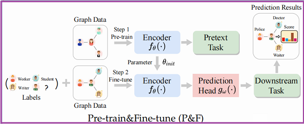
　　首先它是一个两阶段框架，预训练：其中的 Encoder $f_{\theta}(\cdot)$ 是通过代理任务预训练得到的，然后预训练得到的参数 $\theta_{\text {init }} $ 将作为 Encoder  $f_{\theta_{i n i t}}(\cdot) $ 初始化参数；微调阶段，$f_{\theta_{i n i t}}(\cdot) $ 则是在某具体的下游任务，通过投影头$g_{\omega}(\cdot)$ 进行微调。

　　学习目标被表述为：

　　　　$\theta^{*}, \omega^{*}=\underset{(\theta, \omega)}{\text{arg min}} \mathcal{L}_{\text {task }}\left(f_{\theta_{i n i t}}, g_{\omega}\right)$
　　其中：

• • $\theta_{\text {init }}=\arg \min _{\theta} \mathcal{L}_{s s l}\left(f_{\theta}\right)$　　
  • $\mathcal{L}_{\text {task }}$ 和 $\mathcal{L}_{s s l}$ 分别是下游任务的损失函数和自监督预训练任务的损失函数　　

2.4.2  联合训练 Joint Learning

　　框架如下：

　　

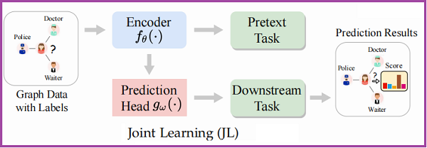
　　在该方案中，Encoder $f_{\theta}(\cdot)$ 在代理任务和下游任务的监督下，与预测头 $g_{\omega}(\cdot) $ 进行联合训练。Joint Learning 策略也可以看作是一种多任务学习，或者将代理任务作为一种正则化学习。学习目标被表述为：

　　　　$\theta^{*}, \omega^{*}=\underset{(\theta, \omega)}{\text{arg min}}   \mathcal{L}_{\text {task }}\left(f_{\theta}, g_{\omega}\right)+\alpha \underset{\theta}{\text{ arg min }}\mathcal{L}_{s s l}\left(f_{\theta}\right)$

　　其中：$\alpha$  是一个 trade-off 参数。

2.4.3  无监督表示学习 Unsupervised Representation Learning

　　框架如下：

　　

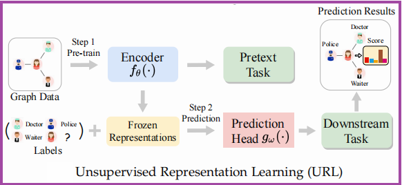
　　这种策略也可以被认为是一个两阶段的方法，第一阶段类似与 Pre-training 框架；第二阶段中输入的不在是图数据而是冻结的表示，通过下游任务进行训练。学习目标被表述为：

　　　　$\omega^{*}=\underset{( \omega)}{\text{arg min}} \mathcal{L}_{\text {task }}\left(f_{\theta_{i n i t}}, g_{\omega}\right)$

　　其中：

• • $\theta_{\text {init }}=\underset{\theta}{\text{arg min}} \mathcal{L}_{s s l}\left(f_{\theta}\right)$　　

　　与其他方案相比，无监督表示学习更具挑战性，因为编码器 $f_{\theta}(\cdot) $ 的学习只依赖于代理任务，并在第二阶段被冻结。相比之下，在P&F策略中，编码器 $f_{\theta}(\cdot) $ 可以在微调阶段的下游任务的监督下进行进一步的优化。