论文解读（GIN）《How Powerful are Graph Neural Networks》

论文信息

论文标题：How Powerful are Graph Neural Networks
论文作者：Keyulu Xu, Weihua Hu, J. Leskovec, S. Jegelka
论文来源：2019, ICLR
论文地址：download 
论文代码：download 

1 Introduction

　　GNN 目前主流的做法是递归迭代聚合一阶邻域表征来更新节点表征，如 GCN 和 GraphSAGE，但这些方法大多是经验主义，缺乏理论去理解 GNN 到底做了什么，还有什么改进空间。

　　GNN 的变体均是遵循两个步骤：邻居聚合（neighborhood aggregation） 和 图池化（graph-level pooling）。　　

　　本文框架受 GNNs 和 WL 图同质测试的启发，若 GNNs 对不同构图能很好识别，则认为是具有较强的表征能力。

　　本文贡献：

• • 证明了GNN最多只和 Weisfeiler-Lehman (WL) test 一样有效，即 WL test 是GNN性能的上限；
  • 建立了邻域聚合（neighbor aggregation）和图读出函数（graph readout functions）的条件，在这些条件下，得到的 GNN 与 WL test 一样强大；
  • 提出图同构网络(Graph Isomorphism Network——GIN)，并证明了它的判别、表征能力等于 WL test 的能力；

2 Preliminaries

2.1 GNN steps

　　GNN 常见的两步走：1、聚合邻居信息；2、更新节点学习

　　GNN 的 第 $k$ 层 表达式：

　　　　$a_{v}^{(k)}=\text { AGGREGATE }^{(k)}\left(\left\{h_{u}^{(k-1)}: u \in \mathcal{N}(v)\right\}\right)$

　　　　$h_{v}^{(k)}=\operatorname{COMBINE}^{(k)}\left(h_{v}^{(k-1)}, a_{v}^{(k)}\right)$

　　AGGREGATE 比较典型的例子是 GraphSAGE：

　　GraphSAGE 的 AGGREGATE 被定义为：

　　　　$a_{v}^{(k)}=\operatorname{MAX}\left(\left\{\operatorname{ReLU}\left(W \cdot h_{u}^{(k-1)}\right), \forall u \in \mathcal{N}(v)\right\}\right)$

 　　这里的 $MAX $ 代表的是 element-wise max-pooling 。

 　　GraphSAGE 的 COMBINE 为 ：

　　　　$W \cdot\left[h_{v}^{(k-1)}, a_{v}^{(k)}\right]$

 　　而在 GCN 中，AGGREGATE 和 COMBINE 集成为：

　　　　$h_{v}^{(k)}=\operatorname{ReLU}\left(W \cdot \operatorname{MEAN}\left\{h_{u}^{(k-1)}, \forall u \in \mathcal{N}(v) \cup\{v\}\right\}\right)$

　　对于节点分类任务，节点表示 $h_{v}^{(K)}$ 将作为预测的输入；对于图分类任务，READOUT 函数聚合了最后一次迭代输出的节点表示$h_{v}^{(K)}$ ，并生成图表示 $h_{G}$ :

　　　　$ h_{G}=\operatorname{READOUT}\left(\left\{h_{v}^{(K)} \mid v \in G\right\}\right)$

　　其中：READOUT 函数是具有排列不变性的函数，如：summation。

2.2 Weisfeiler-Lehman test

　　图同构问题（ graph isomorphism problem）：询问这两个图在拓扑结构上是否相同。

　　WL test  为了辨别多标签图，具体步骤如下：[ 参考《Weisfeiler-Lehman(WL) 算法和WL Test》 ]

• • 迭代地聚合节点及其邻域的标签；
  • 将聚合后的标签散列为唯一的新标签。如果在某次迭代中，两个图之间的节点标签不同，则该算法判定两个图是非同构的；

　　基于 WL test 的多图相似性判别算法 WL subtree kernel 也被提出，图示如下：

　　　　

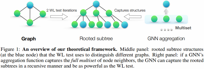
　　上述过程是将 2WL test 保存为树结构。

3 Theoretical framework：overview

　　Definition 1 (Multiset). A multiset is a generalized concept of a set that allows multiple instances for its elements. More formally, a multiset is a 2-tuple  $X=(S, m)$  where  $S$  is the underlying set of  $X$  that is formed from its distinct elements, and  $m: S \rightarrow \mathbb{N}_{\geq 1}$  gives the multiplicity of the elements.

　　假设节点 $v$ 及其邻居集合 $\mathcal{N} (v)$ ，假设节点 $v$ 的标签是 1 ，其 $\mathcal{N} (v)$ 对应的标签是 1、1、2、3、4，可以把邻居集合看成一个 Multiset 。

4 Building powerful graph neural networks

　　作者提出 Theorem 2：即为图同质测试。

　　Lemma 2. Let  $G_{1}$  and  $G_{2}$  be any two non-isomorphic graphs. If a graph neural network  $\mathcal{A}: \mathcal{G} \rightarrow \mathbb{R}^{d}$  maps  $G_{1}$  and  $G_{2}$  to different embeddings, the Weisfeiler-Lehman graph isomorphism test also decides  $G_{1}$  and  $G_{2}$  are not isomorphic.

　　Lemma 2 证明：

　　假设：如果节点标签一致，那么节点表示也一致。

　　假设对节点 $v$ 做了 $k$ 次 WL test 标签聚合，其最终标签若相似，则节点表示也一致。那么如果在 GNN 中，$k$ hop 邻域一样，那么必然节点表示一样。WL test 过程和 GNN 聚合过程是一致的。 

　　作者提出 Theorem 3：如果 GNN 中 Aggregate、Combine 和 Readout 函数是单射，GNN 可以和 WL test 一样强大。

　　Theorem 3. Let  $\mathcal{A}: \mathcal{G} \rightarrow \mathbb{R}^{d}$  be a  GNN . With a sufficient number of GNN layers,  $\mathcal{A}$  maps any graphs  $G_{1}$  and  $G_{2}$  that the Weisfeiler-Lehman test of isomorphism decides as non-isomorphic, to different embeddings if the following conditions hold:

　　 a) A aggregates and updates node features iteratively with

　　　　$h_{v}^{(k)}=\phi\left(h_{v}^{(k-1)}, f\left(\left\{h_{u}^{(k-1)}: u \in \mathcal{N}(v)\right\}\right)\right)$

　　     where the functions $f$,  which operates on multisets, and $\phi$ are injective(单射). 

 　　b)  $\mathcal{A}$'s graph-level readout, which operates on the multiset of node features $\left\{h_{v}^{(k)}\right\}$ , is injective. 

　　Theorem 3 证明和 Lemma2 证明思想类似，都是基于相同假设。

4.1 Graph isomorphism network(GIN)

　　为建模邻居聚合的单射多集函数。

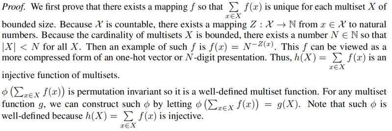
　　下述 Lemma 5 阐述 sum aggregators 是单射的：

　　Lemma 5. Assume $\mathcal{X}$ is countable. There exists a function $f: \mathcal{X} \rightarrow \mathbb{R}^{n}$ so that $h(X)=\sum_{x \in X} f(x)$ is unique for each multiset $X \subset \mathcal{X}$ of bounded size. Moreover, any multiset function $g$ can be decomposed as $g(X)=\phi\left(\sum\limits _{x \in X} f(x)\right)$ for some function $\phi $.

　　Lemma5 证明：

　　出发点：考虑一个有 $N$ 个 元素的 multiset ，对其进行任意划分，最多可以划分成 $N$ 个子集，所以很自然的可以使用 $N$ 个正整数对其打上唯一标记，因此证明 $f$ 可以是唯一的单射函数。

　　

　　Corollary 6. Assume  $\mathcal{X}$  is countable. There exists a function  $f: \mathcal{X} \rightarrow \mathbb{R}^{n}$  so that for infinitely many choices of  $\epsilon$ , including all irrational numbers,  $h(c, X)=(1+\epsilon) \cdot f(c)+\sum\limits _{x \in X} f(x)$  is unique for each pair  $(c, X)$ , where  $c \in \mathcal{X}$  and  $X \subset \mathcal{X}$  is a multiset of bounded size. Moreover, any function $g$ over such pairs can be decomposed as $ g(c, X)=\varphi\left((1+\epsilon) \cdot f(c)+\sum\limits_{x \in X} f(x)\right)$  for some function  $\varphi $.

　　Corollary 6 证明：

　　

　　对于第一种情况利用 Lemma 5 解释，对于第二种情况利用无理数 $\epsilon$ 的性质。

　　Corollary 6 证明了 $ h(c, X)=(1+\epsilon) \cdot f(c)+\sum\limits_{x \in X} f(x)$ 是单射函数，同时本文也将 $\varphi$ 和 $f$ 用 MLP 代替（由于 MLP 是万能近似函数，可以模拟单射性质），又根据单射的性质  （若 $f$ 和 $g$ 皆为单射的，则 $f o g$ 亦为单射），得 $MLP(h(c, X))$ 也是单射的，即：

　　　　$h_{v}^{(k)}=\operatorname{MLP}^{(k)}\left(\left(1+\epsilon^{(k)}\right) \cdot h_{v}^{(k-1)}+\sum\limits _{u \in \mathcal{N}(v)} h_{u}^{(k-1)}\right)  \quad\quad\quad({\large \star } )$

4.2 Graph-level readout of GIN 

　　Readout 模块使用 concat+sum，对每次迭代得到的所有节点特征求和得到图的特征，然后拼接起来。

　　　　$h_{G}=\operatorname{CONCAT}\left(\operatorname{READOUT}\left(\left\{h_{v}^{(k)} \mid v \in G\right\}\right) \mid k=0,1, \ldots, K\right)$

　　即

　　　　$h_{G}=\operatorname{CONCAT}\left(\operatorname{sum}\left(\left\{h_{v}^{(k)} \mid v \in G\right\}\right) \mid k=0,1, \ldots, K\right)$

5 Less powerful but still interesting GNNs

 　　本文研究不满足 Theorem 3 的 GraphSAGE 和 GCN，做了两个消融实验：

• • 1-layer perceptrons instead of MLPs .　　
  • mean or max-pooling instead of the sum.　　

5.1 1-layer perceotrons are not sufficient

　　许多GNN 任然采用 1 层的 perceptrons，对于某些 multiset 可能存在无法区别的问题。

　　Lemma 7. There exist finite multisets  $X_{1} \neq X_{2}$  so that for any linear mapping  $W $,  ${\small \sum\limits_{x \in X_{1}} \operatorname{ReLU}(W x)=\sum\limits_{x \in X_{2}} \operatorname{ReLU}(W x)} $.

　　Lemma 7 证明：

　　

　　1 层的 perceptrons 表现得很像线性映射，因此 GNN 层退化为对邻域特征的简单求和。本文的证明建立在线性映射中缺乏偏差项这一事实之上。有了偏差项和足够大的输出维数，1 层的 perceptrons 可能能够区分不同的 multiset。

5.2 Structures that confuse mean and max-pooling

　　现在考虑将 $h(X)=\sum\limits _{x \in X} f(x)$ 中的 sum 替换为 Mean-pooling 和 Max-pooling 将产生什么问题。

　　Mean-pooling 和 max-pooling aggregators 在某种程度上是一种好的 multiset functions [ 具有平移不变性 ]，但是他们不是单射的。

　　Figure 2 根据三个 aggregators 的表示能力进行了排序。

　　　　

　　三种不同的 Aggregate：

• • sum：学习全部的标签以及数量，可以学习精确的结构信息（不仅保存了分布信息，还保存了类别信息）；[ 蓝色：4个；红色：2 个  ] 
  • mean：学习标签的比例（比如两个图标签比例相同，但是节点有倍数关系），偏向学习分布信息；[ 蓝色：$4/6=2/3$ 的比例；红色：$2/6=1/3$ 的比例  ] 
  • max：学习最大标签，忽略多样，偏向学习有代表性的元素信息；[ 两类（类内相同），所以各一个  ] 

　　Figure 3 说明了mean-pooling aggregators 和 max-pooling aggregators 无法区分的结构对。 

　　　　

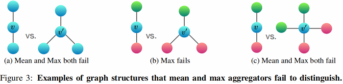
　　在 Figure 3a 中：Every node has the same feature $a$ and $f(a)=h_a$ is the same across all nodes.

• • mean：左 $\frac{1}{2}(h_a+h_a)=h_a$ ，右：$\frac{1}{3}(h_a+h_a+h_a)=h_a$，无法区分；
  • max：左 $h_a$ , 右 $h_a$ 无法区分；
  • sum：左 $2h_a$ , 右 $3h_a$ , 可以区分；

　　在 Figure 3b 中：Let $h_{\text {color }}(r \text { for red, } g \text { for green })$ denote node features transformed by $f $. 

• • mean: 左 $ \frac{1}{2}(h_r+h_g)$ ，右： $\frac{1}{3}(h_g+2h_r) $ ，可以区分；
  • max : 左 $max (h_r, h_g) $ ，右： $max (h_g, h_r, h_r) $ ，无法区分;
  • sum: 左 $sum(h_r+h_g)$ , 右 $sum(2 h_r+h_g)$ , 可以区分；

　　在 Figure 3c 中：

• • mean：左 $\frac{1}{2}(h_r+h_g) $ ，右：$\frac{1}{4}(2 h_g+2 h_r) $ ，无法区分;
  • max：左 $\max (h_g, h_g, h_r, h_r)$ ，右：$\max (h_g, h_r)$ ，无法区分；
  • sum：左 $h_r+h_g$ ，右：$2 h_r+2 h_g$ ，可以区分；

5.3 Mean learns distrubutions

 　　旨在说明等比例 multiset ，使用 mean 是无法区分的。

　　Corollary 8. Assume  $\mathcal{X}$  is countable. There exists a function  $f: \mathcal{X} \rightarrow \mathbb{R}^{n}$  so that for  $h(X)=   \frac{1}{|X|} \sum\limits _{x \in X} f(x), h\left(X_{1}\right)=h\left(X_{2}\right)$  if and only if multisets  $X_{1}$  and  $X_{2}$  have the same distribution. That is, assuming  $\left|X_{2}\right| \geq\left|X_{1}\right| , we have  X_{1}=(S, m)$  and  $X_{2}=(S, k \cdot m)$  for some $k \in \mathbb{N}_{\geq 1}$ .

5.4 Max-pooling learns sets with distinct elements

　　Max-pooling 阐述的是，只要决定性元素（max value）一样，其他元素是否考虑无关紧要。显然这是不合理的。

　　Corollary 9. Assume  $\mathcal{X}$  is countable. Then there exists a function  $f: \mathcal{X} \rightarrow \mathbb{R}^{\infty}$  so that for  ${\small h(X)=\underset{x \in X}{max} f(x), h\left(X_{1}\right)=h\left(X_{2}\right)} $  if and only if  $X_{1}$  and  $X_{2}$  have the same underlying set.

6 Experiments

6.1 Training set performance of GINs

　　　　

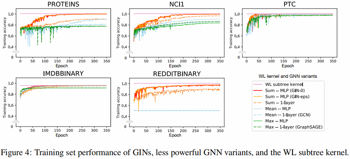
　　在训练中，GIN 和WL test 一样，可以拟合所有数据集，这表说了 GIN 表达能力达到了上限

6.2 Generalization ability of GNNs

　　　　

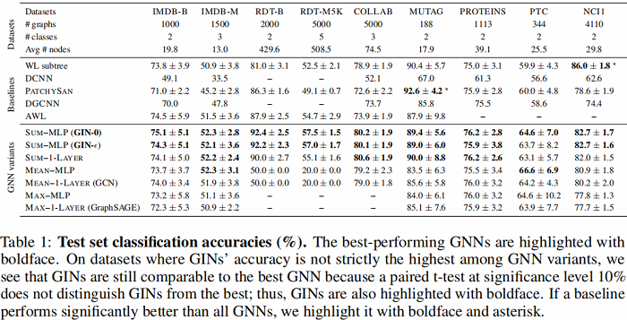
• • GIN-0 比GIN-eps 泛化能力强：可能是因为更简单的缘故；
  • GIN 比 WL test 效果好：因为GIN进一步考虑了结构相似性，即WL test 最终是one-hot输出，而GIN是将WL test映射到低维的embedding；
  • max 在无节点特征的图（用度来表示特征）基本无效；

7 Conclusion

　　本文主要 基于对 graph分类，证明了 sum 比 mean 、max 效果好，但是不能说明在node 分类上也是这样的效果，另外可能优先场景会更关注邻域特征分布， 或者代表性， 故需要都加入进来实验。

 

修改历史

2021-03-15 创建文章
2022-06-10 修订文章，大整理

 

论文解读目录