论文解读(SDNE)《Structural Deep Network Embedding》
论文信息
论文标题:Structural Deep Network Embedding
论文作者:Aditya Grover;Aditya Grover; Jure Leskovec
论文来源:2016, KDD
论文地址:download
论文代码:download
1 Introduction
网络表示学习,可以用于学习网络节点的向量表示,从而表示网络结构等信息。目前几乎所有的网络表示学习方法都是基于浅层模型,但由于网络结构本身比较复杂,浅层模型往往收敛于局部最优解,无法表示更高级的非线性网络结构。
本文作者基于此,提出SDNE模型(Structure Deep Network Embedding),模型可以有效提取网络局部和全局结构信息。
SDNE 属于一个 半监督模型。
-
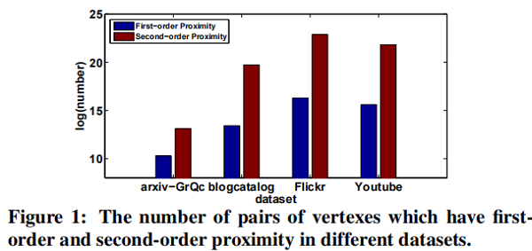
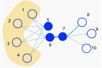
- The second-order proximity is used by the unsupervised component to capture the global network structure.
- The first-order proximity is used as the supervised information in the supervised component to preserve the local network structure.
网络表示学习遇到的挑战:
- High non-linearity: the underlying structure of the network is highly non-linear.
- Structure-preserving: The underlying structure of the network is very complex. The similarity of vertexes is dependent on both the local and global network structure. Therefore, how to simultaneously preserve the local and global structure is a tough problem.
- Sparsity: Many real-world networks are often so sparse that only utilizing the very limited observed links is not enough to reach a satisfactory performance .
2 Structural deep network embedding
2.1 Framework
一个 semi-supervised 的深度模型,其框架如图 Figure 2 所示.
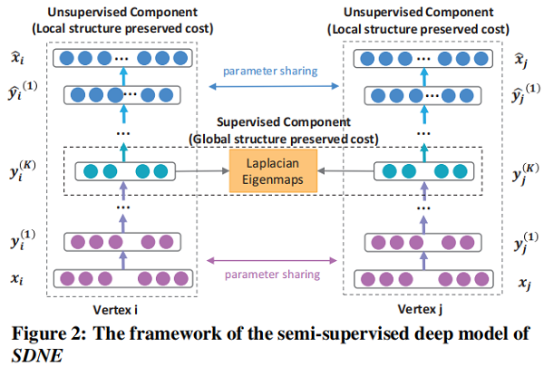
2.2 Loss Functions
本文定义如 Table 1 所示:
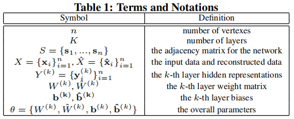
给定输入 $ x_i$,自编码器每层的节点表示为 :
$\begin{array}{l}\mathbf{y}_{i}^{(1)}=\sigma\left(W^{(1)} \mathbf{x}_{i}+\mathbf{b}^{(1)}\right) \\\mathbf{y}_{i}^{(k)}=\sigma\left(W^{(k)} \mathbf{y}_{i}^{(k-1)}+\mathbf{b}^{(k)}\right), k=2, \ldots, K\end{array}\quad \quad \quad \quad (1)$
获得 $\mathbf{y}_{i}^{(K)}$ 后 , 计算重构误差:
$\mathcal{L}=\sum \limits _{i=1}^{n}\left\|\hat{\mathbf{x}}_{i}-\mathbf{x}_{i}\right\|_{2}^{2}$
本文使用邻接矩阵 $S$ 作为自编码器的输入,即 $x_i = s_i$ ,由于每个实例 $s_i$ 表征了顶点 $v_i$ 的邻域结构,重建过程将使具有相似邻域结构的顶点具有相似的邻域结构潜在表征。
通过分析,不能直接使用 $S$ 矩阵,因为网络的稀疏性,$S$ 中非零元素的数量远远少于零元素的数量。 如果直接使用 $S$ 作为自编码器的输入,则更容易重构 $S$ 中的零元素,即出现很多 $0$ 元素。
为解决上述问题,我们对非零元素的重构误差施加了比零元素更大的惩罚,修正后的目标函数如下所示:
$\begin{aligned}\mathcal{L}_{2 n d} &=\sum \limits _{i=1}^{n}\left\|\left(\hat{\mathbf{x}}_{i}-\mathbf{x}_{i}\right) \odot \mathbf{b}_{\mathbf{i}}\right\|_{2}^{2} \\&=\|(\hat{X}-X) \odot B\|_{F}^{2}\end{aligned}\quad \quad \quad \quad (3)$
其中
-
- $\odot$ 表示 Hadamard 积;
- $\mathbf{b}_{\mathbf{i}}=\left\{b_{i, j}\right\}_{j=1}^{n}$ ,如果 $s_{i, j}= 0, b_{i, j}=1$ ,否则 $b_{i, j}=\beta>1$
现在,通过使用以邻接矩阵 $S$ 作为输入的修改后的深度自动编码器,具有相似邻域结构的顶点将被映射到表示替换中的附近。 SDNE 的 Unsupervised Component 可以通过重建顶点之间的二阶接近度来保留全局网络结构。
为捕捉局部结构,使用一阶邻近度来表示局部网络结构。设计 supervised component 以利用一阶接近度。损失函数定义如下:
$\begin{aligned}\mathcal{L}_{1 s t} &=\sum \limits _{i, j=1}^{n} s_{i, j}\left\|\mathbf{y}_{i}^{(K)}-\mathbf{y}_{j}^{(K)}\right\|_{2}^{2} \\&=\sum \limits _{i, j=1}^{n} s_{i, j}\left\|\mathbf{y}_{i}-\mathbf{y}_{j}\right\|_{2}^{2}\end{aligned} \quad \quad \quad \quad (4)$
其中 $\mathcal{L}_{\text {reg }}$ 是一个 $\mathcal{L}$ 2-norm 正则化项,用于防止过拟合,其定义如下:
$\mathcal{L}_{r e g}=\frac{1}{2} \sum \limits_{k=1}^{K}\left(\left\|W^{(k)}\right\|_{F}^{2}+\left\|\hat{W}^{(k)}\right\|_{F}^{2}\right)$
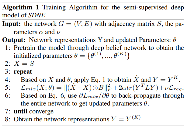
2.3 Optimization
为优化上述模型,目标是最小化关于 $\theta$ 的 $\mathcal{L}_{\operatorname{mix}}$ 函数。详细地说,关键步骤是计算偏导数(partial derivative)$\partial \mathcal{L}_{m i x} / \partial \hat{W}^{(k)}$ 和 $ \partial \mathcal{L}_{\operatorname{mix}} / \partial W^{(k)}$ :
$\begin{array}{l}{\large \frac{\partial \mathcal{L}_{m i x}}{\partial \hat{W}^{(k)}}=\frac{\partial \mathcal{L}_{2 n d}}{\partial \hat{W}^{(k)}}+\nu \frac{\partial \mathcal{L}_{r e g}}{\partial \hat{W}^{(k)}} \\\frac{\partial \mathcal{L}_{m i x}}{\partial W^{(k)}}=\frac{\partial \mathcal{L}_{2 n d}}{\partial W^{(k)}}+\alpha \frac{\partial \mathcal{L}_{1 s t}}{\partial W^{(k)}}+\nu \frac{\partial \mathcal{L}_{r e g}}{\partial W^{(k)}}, k=1, \ldots, K} \end{array}\quad \quad \quad \quad (6)$
首先来看 $\partial \mathcal{L}_{2 n d} / \partial \hat{W}^{(K)}$ :
$ {\large \frac{\partial \mathcal{L}_{2 n d}}{\partial \hat{W}^{(K)}}=\frac{\partial \mathcal{L}_{2 n d}}{\partial \hat{X}} \cdot \frac{\partial \hat{X}}{\partial \hat{W}^{(K)}}} \quad \quad \quad \quad (7)$
对于第一项,根据 Eq. 3,有:
${\large \frac{\partial \mathcal{L}_{2 n d}}{\partial \hat{X}}=2(\hat{X}-X) \odot B } \quad \quad \quad \quad (8)$
第二项的计算 $\partial \hat{X} / \partial \hat{W}$ 可由 $\hat{X}=$ $\sigma\left(\hat{Y}^{(K-1)} \hat{W}^{(K)}+\hat{b}^{(K)}\right) $ 计算。 然后 $\partial \mathcal{L}_{2 n d} / \partial \hat{W}^{(K)}$ 可以计算出。基于反向传播,我们可以迭代地得到 $\partial \mathcal{L}_{2 n d} / \partial \hat{W}^{(k)}, k=$ $1, \ldots K-1$ 和 $\partial \mathcal{L}_{2 n d} / \partial W^{(k)}, k=1, \ldots K $ 。现在 $\mathcal{L}_{2 n d}$ 的偏导数计算完成。
现在计算 $\partial \mathcal{L}_{1 s t} / \partial W^{(k)}$. $\mathcal{L}_{1 s t}$ 可以表述为:
$\mathcal{L}_{1 s t}=\sum_{i, j=1}^{n} s_{i, j}\left\|\mathbf{y}_{i}-\mathbf{y}_{j}\right\|_{2}^{2}=2 \operatorname{tr}\left(Y^{T} L Y\right) \quad \quad \quad \quad (9)$
其中 $L=D-S, D \in \mathbb{R}^{n \times n}$ 是 diagonal matrix,$D_{i, i}=$ $\sum_{j} s_{i, j} $ 。
然后首先关注计算 $\partial \mathcal{L}_{1 s t} / \partial W^{(K)}$ :
$\frac{\partial \mathcal{L}_{1 s t}}{\partial W^{(K)}}=\frac{\partial \mathcal{L}_{1 s t}}{\partial Y} \cdot \frac{\partial Y}{\partial W^{(K)}} \quad \quad \quad \quad (10)$
因为 $Y=\sigma\left(Y^{(K-1)} W^{(K)}+b^{(K)}\right)$, 第二项 $\partial Y / \partial W^{(K)}$ 可容易计算出。对于第一项 $\partial \mathcal{L}_{1 s t} / \partial Y$,我们有:
$\frac{\partial \mathcal{L}_{1 \text { st }}}{\partial Y}=2\left(L+L^{T}\right) \cdot Y \quad \quad \quad \quad (11)$
同样地,利用反向传播,我们可以完成对的 $\mathcal{L}_{1 s t}$ 偏导数的计算。
现在我们得到了这些参数的偏导数。通过对参数的初始化,可以利用 $SGD$ 对所提出的深度模型进行优化。需要注意的是,由于模型的非线性较高,在参数空间中存在许多局部最优。因此,为了找到一个良好的参数空间区域,我们首先使用 Deep Belief Network 对参数进行 pretrain ,这在文献中被证明是深度学习的必要参数初始化。
3 Experiments
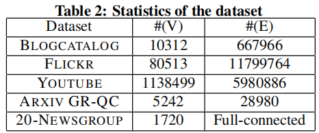
数据集
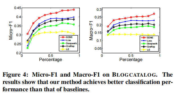
Multi-label Classification
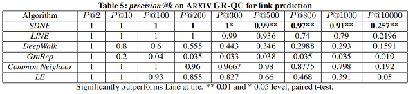
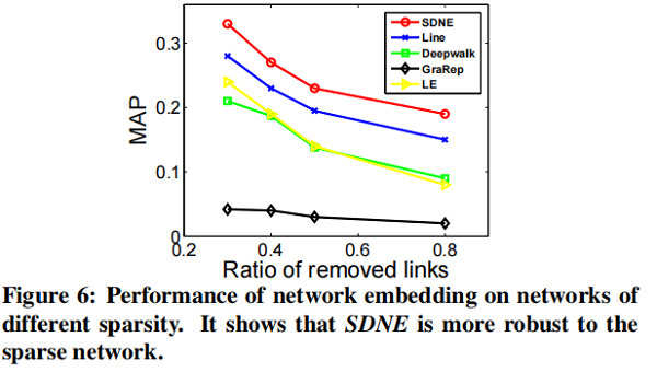
Link Prediction
在本节中,我们将专注于 link prediction task ,并进行了两个实验。第一种评估整体性能,第二种评估网络的不同稀疏性如何影响不同方法的性能。
我们随机隐藏部分现有的链路,并使用网络来训练网络嵌入模型。训练结束后,我们可以得到每个顶点的表示,然后使用所得到的表示来预测未被观察到的链接。
可视化


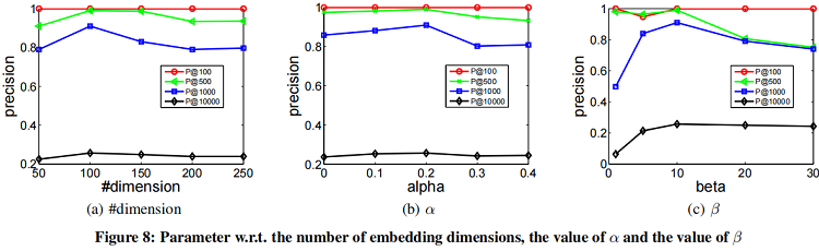
参数敏感性实验
4 Conclusion
使用自编码器重构一阶接近度和二阶接近度。
修改历史
2021-12-06 创建文章
2022-06-08 修订文章
因上求缘,果上努力~~~~ 作者:别关注我了,私信我吧,转载请注明原文链接:https://www.cnblogs.com/BlairGrowing/p/15622594.html

 浙公网安备 33010602011771号